@GLSDetrend is a local-to-unity detrending routine allowing for various types of trends, including ones with a break at a known point. This includes the Elliott-Rothenberg-Stock cases (no constant, constant, constant and trend) as well as the Perron and Rodriguez cases (constant and trend with a single break). This just does the detrending, not the actual unit root test(s). For models with breaks, you need to input the break point.

@GLSDetrend( options ) y start end yd

Parameters

Options

DET=NONE/[CONSTANT]/TREND

BREAK=[NONE]/INTERCEPT/TREND/BOTH

Note - Perron and Rodriguez don't include the case with just a break in the intercept.

 

TB=entry for break

This is required if any of the BREAK choices are used. The dummies are (t>TB) for the intercept and max(t-TB,0) for the trend, so the structure is different at TB+1 than at TB.

 

CBAR=(positive) determines GLS \(\rho\) value as \(\rho=1-\text{cbar}/T\) [depends upon model]

 

U/[NOU]

U indicates unconditional distribution (for U0) is to be used

Variables Defined

The standard regression variables can be used. The regressors are in order 1, t, intercept break dummy, trend break dummy

 

Example

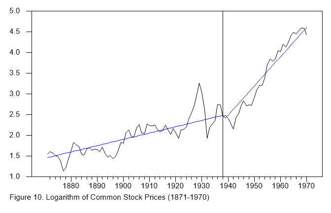
This does a GLS detrending with break at 1938:1 for the log stock price data from the Nelson-Plosser data set. It subtracts the detrended data from the original to get the trend itself, and graphs the series along with the extracted trend.

 

open data nelsonplosser.rat

calendar(a) 1871

data(format=rats) 1871:1 1970:1 realwages stockprice

*

set logwage  = log(realwages)

set logstock = log(stockprice)

*

@glsdetrend(break=both,tb=1938:1) logstock / stockdetrend

set stocktrend = logstock-stockdetrend

graph(footer="Figure 10. Logarithm of Common Stock Prices (1871-1970)",grid=(t==1938:1)) 2

# logstock

# stocktrend

Sample Graph

This is the graph generated by the example. Again, note that the trend itself is created by subtracting the detrended series produced by the procedure from the original data.

 

 

Copyright © 2025 Thomas A. Doan