@ICSS does the procedure for searching for breaks in variance using the algorithm described in Inclan and Tiao(1994). The underlying assumption is that the input data has a common mean, but possibly different variances within subsamples. Because this is doing a search for breaks, the test statistic has a non-standard distribution—the procedure takes the significance level (or critical value) as an input and searches for break points where the variance is significantly different before and after those points.

 

The original algorithm is based upon an assumption that the data are Normally distributed. Sanso, Arago and Carrion-i-Silvestre(2004) generalized this to allow for an estimated 4th moment (rather than using the implied 4th moment under the assumption of normality). You can get this variant by using the ROBUST option.

@ICSS( options )   x start end

Parameters

Options

SIGNIF=.01/[.05]/.10

CV=critical value for determining variance change [not used]

This determines the critical value used for determining whether a subsample split should be accepted. If CV isn't used, the SIGNIF option controls (with a default of .05), which uses the asymptotic critical values (1.358 for .05, 1.628 for .01 and 1.224 for .10). CV can be used for inputting a specific alternative value.

 

ROBUST/[NOROBUST]

If ROBUST, corrects the statistics for a non-Gaussian distribution (using sample estimates of the 4th moment).

 

BREAKS=(output) VECT[INT] of entries with breaks located [not used]

SUBSAMPLES=(output) RECT[INT] with subsamples [not used]

For the array created by SUBSAMPLES, ss(1,i) is the start entry of the ith subsample and ss(2,i) is the end entry.

Note that there if there are K breaks, there will be K+1 subsamples. A breakpoint marks the end of a subsample.

 

[PRINT]/NOPRINT

TITLE=title for report ["ICSS Analysis of Series ..."

 

TRACE/[NOTRACE]

If TRACE, information is presented showing the decisions taken in coming up with sample breaks.

Example

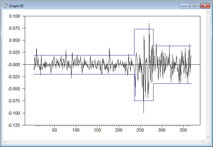
This is based upon the example from the original Inclan and Tiao paper. It identifies the variance breaks using the default .05 significance level and graphs the data with +/- 2 standard deviation bands.

 

*

* Replication file for Inclan and Tiao, "Use of Cumulative Sums of

* Squares for Retrospective Detection of Changes in Variance", JASA

* 1994, vol 89, pp 913-923

*

* Note that the entry numbers are off by one from those given in the

* article. This is because RATS is basing entry numbers on the start of

* the original stock price series, not on the start of the log

* differenced data.

*

data(unit=input) 1 369 ibm

 460 457 452 459 462 459 463 479 493 490 492 498 499 497 496

 490 489 478 487 491 487 482 479 478 479 477 479 475 479 476

 476 478 479 477 476 475 475 473 474 474 474 465 466 467 471

 471 467 473 481 488 490 489 489 485 491 492 494 499 498 500

 497 494 495 500 504 513 511 514 510 509 515 519 523 519 523

 531 547 551 547 541 545 549 545 549 547 543 540 539 532 517

 527 540 542 538 541 541 547 553 559 557 557 560 571 571 569

 575 580 584 585 590 599 603 599 596 585 587 585 581 583 592

 592 596 596 595 598 598 595 595 592 588 582 576 578 589 585

 580 579 584 581 581 577 577 578 580 586 583 581 576 571 575

 575 573 577 582 584 579 572 577 571 560 549 556 557 563 564

 567 561 559 553 553 553 547 550 544 541 532 525 542 555 558

 551 551 552 553 557 557 548 547 545 545 539 539 535 537 535

 536 537 543 548 546 547 548 549 553 553 552 551 550 553 554

 551 551 545 547 547 537 539 538 533 525 513 510 521 521 521

 523 516 511 518 517 520 519 519 519 518 513 499 485 454 462

 473 482 486 475 459 451 453 446 455 452 457 449 450 435 415

 398 399 361 383 393 385 360 364 365 370 374 359 335 323 306

 333 330 336 328 316 320 332 320 333 344 339 350 351 350 345

 350 359 375 379 376 382 370 365 367 372 373 363 371 369 376

 387 387 376 385 385 380 373 382 377 376 379 386 387 386 389

 394 393 409 411 409 408 393 391 388 396 387 383 388 382 384

 382 383 383 388 395 392 386 383 377 364 369 355 350 353 340

 350 349 358 360 360 366 359 356 355 367 357 361 355 348 343

 330 340 339 331 345 352 346 352 357

*

set ldiff = log(ibm/ibm{1})

@ICSS(subsamples=ss) ldiff 2 369

*

* Pull the common mean out of the data.

*

diff(center) ldiff / demean

compute mean=%mean

*

* Compute the variance (sum of squares/T) for each of the subsamples,

* and create upper and lower 2 standard deviation bounds (relative to

* the common mean).

*

do i=1,%cols(ss)

   sstats(mean) ss(1,i) ss(2,i) demean^2>>svar

   set upper ss(1,i) ss(2,i) = mean+2.0*sqrt(svar)

   set lower ss(1,i) ss(2,i) = mean-2.0*sqrt(svar)

end do i

*

graph(overlay=step,ovcount=2,ovsame) 3

# ldiff

# upper / 2

# lower / 2

 

Sample Output

 

ICSS Analysis of Series LDIFF

Using significance level 0.05

Breakpoints found at entries

236

280

 

 

Copyright © 2025 Thomas A. Doan