@LSUNIT implements a variety of LM unit root tests allowing for 0, 1, 2 or even more structural breaks of one of two varieties, as described in Lee and Strazicich(2003). This point of this (and similar) tests is widely misunderstood. See Unit Roots and Breaks.

 

This can take a very long time for two or more breaks if the data set is large (>500 observations). The calculation time goes up with T^(# of breaks+1), so with 1000 data points, you're looking at roughly 1000 times as long to do two breaks as one. You can use the THIN option to reduce the computational burden for large data sets.
 

@LSUNIT and other similar procedures are used in the UNITROOTBREAK.RPF example to test for unit roots.

 

@LSUNIT(options)   series start end

Wizards

This is included as one of the tests in the Time Series—Unit Root Test Wizard.

Parameters

Options

MODEL=[CRASH]/BREAK

Model of structural break. MODEL=CRASH has an abrupt change in level, but no change in the trend rate. MODEL=BREAK allows for (simultaneous) changes in level and trend. In general, only one is likely to be of interest for a particular series, which you can determine by graphing the series.

 

BREAKS=Number of breaks [1]

Number of breaks. This allows for any positive number, but note that tables of critical values exist only for 0, 1 and 2. The programming for 3 or more breaks is effectively the same as for 2, which is why we allow for it. Whether there is any actual value in that many breaks is unclear.

 

LAGS=number of lags on the auxiliary regression [1]

METHOD=[FIXED]/GTOS

SLSTAY=significance level to keep lag in model with METHOD=GTOS [.10]

If METHOD=FIXED, the number of lags on the LAGS option is included in all regressions. If METHOD=GTOS (general-to-specific), lags are dropped from the end so long as the significance level of the t-statistic is greater than the SLSTAY value.

 

PI=fraction of entries on each end of data to exclude as break points, and minimum gap between breakpoints [.10]

THIN=entry spacing on the grid of data points [1]

With the default of THIN=1, every possible set of breaks that are separated as given by the PI option are examined. As described above, this can take a great deal of time on a large data set if you're looking for 2 or more breaks. A higher value for the THIN option (for example THIN=5) can reduce that time by only looking at every 5th entry for each possible break.
 

[PRINT]/NOPRINT

TITLE=title for report ["Lee-Strazicich Unit Root Test, Series ..."

Variables Defined

Notes

This differs slightly from Lee and Strazicich's Gauss code as the lag pruning regressions use a common estimation range (from maxlag+1 on) rather than the lag+1 samples used in the Gauss code. The method chosen here would make it simpler to change the pruning method to an alternative like minimum AIC.

 

The critical values for MODEL=CRASH are independent of the locations of the breaks, but the critical values for MODEL=BREAK depend upon the (approximate) locations of the break(s) (as a percentage of the entry range). @LSUnit greatly expands upon the set of pairs for which approximate critical values have been computed (versus the ones in the Lee-Strazicich papers). For one break, the critical values are tabulated for \(\lambda\)=.10,.15,...,.50 (with symmetry around .5) and are linearly interpolated from those based upon the observed location. For two breaks, the critical values are tabulated for pairs of (differing) values from \(\lambda\)=.20,.30,...,.80. (The time required to simulate double breaks is quite high, hence the much coarser grid). The pair closest to the observed breaks is used (again, symmetry of the pair around .5 is used, that is, .6,.8 has the same critical value as .2,.4).

Example

cal(a) 1960

data(format=free,unit=input,org=cols) 1 38 year x

1960    11508

1961    11369

1962    11930

1963    12636

1964    13194

1965    13264

1966    13875

1967    14193

1968    15172

1969    15712

1970    16316

1971    16872

1972    17563

1973    18489

1974    18606

1975    18741

1976    18728

1977    18480

1978    19303

1979    19682

1980    19968

1981    20271

1982    19464

1983    20127

1984    20712

1985    21438

1986    21719

1987    22443

1988    23040

1989    22995

1990    22226

1991    21921

1992    22367

1993    23176

1994    24144

1995    24818

1996    25077

1997    25608

set logx = log(x)

graph

# logx

@lsunit(breaks=0,lags=5,method=gtos) logx

@lsunit(breaks=2,pi=.10,lags=5,method=gtos,model=crash) logx

@lsunit(breaks=2,pi=.10,lags=5,method=gtos,model=break) logx

Sample Output

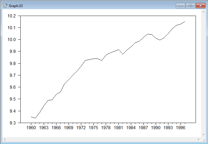
This does a "no break" test (basically Schmidt-Phillips with a linear trend) and then two break tests in each form. In all cases, the test statistic is the t-statistic on S{1}. The first test rather easily accepts the unit root. (A Dickey-Fuller test allowing for trend would give a similar result). If you look at the data, there appears to be a fairly clear change in the rate of growth starting in roughly 1973 and a couple of possible "crash" breaks (drop with no real change in growth rate) later in the data set. Since the crash model doesn't admit a change in the growth rate, it's not the test form that's really compatible with the data, but we'll include it as an example.

 

Both the LS tests would accept the hypothesis of a unit root allowing for breaks. Note, however, that the crash model accepts the null despite having a very negative t-statistic and a coefficient on S{1} that's nowhere near zero—with so few data points, the test won't have much power.

 

Note that the locations of the breaks (1971:1 and 1981:1 for the crash model and 1970:1 and 1990:1 for the break model) don't really correspond to the date of the break that would seem to be appropriate from looking at the data. This is another reminder that this is not a test for breaks—it's a test for unit roots allowing for breaks, and the break locations are chosen to give the most negative test statistic, not the best fit to the data.

 

Lee-Strazicich Unit Root Test, Series LOGX

Regression Run From 1966:01 to 1997:01

Observations          32

No Breaks - Schmidt-Phillips Test

With 5 lags chosen from 5

                                     Critical Values

Variable     Coefficient T-Stat  .01     .05     .10

S{1}             -0.1509 -1.8326 -3.5970 -3.0310 -2.7450

Constant          0.0339  4.2690

 

Lee-Strazicich Unit Root Test, Series LOGX

Regression Run From 1966:01 to 1997:01

Observations          32

Crash Model with 2 breaks

With 5 lags chosen from 5

                                     Critical Values

Variable     Coefficient T-Stat  .01     .05     .10

S{1}             -0.2465 -2.6392 -4.0730 -3.5630 -3.2960

Constant          0.0398  5.3408

D(1971:01)        0.0269  1.2696

D(1981:01)       -0.0387 -1.7997

 

Lee-Strazicich Unit Root Test, Series LOGX

Regression Run From 1966:01 to 1997:01

Observations          32

Trend Break Model with 2 breaks

With 2 lags chosen from 5

                                     Critical Values

Variable     Coefficient T-Stat  .01     .05     .10

S{1}             -1.0983 -5.1986 -6.6910 -6.1520 -5.7980

Constant          0.0198  2.4096

D(1970:01)       -0.0152 -0.8670

DT(1970:01)       0.0272  2.0811

D(1990:01)       -0.0146 -0.7537

DT(1990:01)      -0.0119 -1.3742

 

Graph of Sample Data

 

Copyright © 2025 Thomas A. Doan