ARMAGIBBS.RPF

ARMAGIBBS.RPF is an example of an analysis of an ARMA(1,1) model using Gibbs sampling (or more accurately, Independence Chain Metropolis-Hastings). This uses a "flat" prior on the coefficients other than restricting them to the interval (-1,1).

Independence Chain M-H requires keeping track of both the posterior (the likelihood here since the prior is flat) and the density function at the last accepted draw. Those are LOGPLAST and LOGQLAST. The sampler is started at the maximum likelihood estimates and the proposal density uses those as the mean and the estimated covariance matrix out of BOXJENK as the covariance matrix.

It does 2500 burn-in and 10000 keeper draws. It saves the full set of ARMA model coefficients, thus the CONSTANT, AR(1) and MA(1) coefficients in that order into the SERIES[VECT]BGIBBS.

Full Program

open data agquarterly.xls
calendar(q) 1960:1
data(format=xls,org=columns) 1960:1 2002:1 ppi
graph(header="Producer Price Index, 1995=100")
# ppi
*
set logppi = log(ppi)
*
boxjenk(diffs=1,constant,ar=1,ma=1,maxl) logppi
*
* The proposal density will be the asymptotic distribution from maximum
* likelihood, thus, the mean is %BETA and the factor of the covariance
* matrix is %SEESQ*%XX. We're also starting the sampling from these
* estimates, so LOGPLAST is %LOGL (we're using a non-informative prior)
* and LOGQLAST is 0.
*
compute bboxj=%beta
compute fxx =%decomp(%seesq*%xx)
compute logplast=%logl
compute logqlast=0.0
compute bdraw=bboxj
*
compute nburn =2500
compute ndraws=10000
*
dec series[vect] bgibbs
gset bgibbs 1 ndraws = %zeros(%nreg,1)
*
compute accept=0
infobox(action=define,lower=-nburn,upper=ndraws,progress) "Independence Metropolis"
do draw=-nburn,ndraws
   *
   * Draw the proposal and save the log kernel for the draw
   *
   compute [vect] btest=bboxj+%ranmvt(fxx,10.0)
   compute logqtest=%ranlogkernel()
   *
   * Reject if AR or MA coefficient is out of range.
   *
   if abs(btest(2))>=1.0.or.abs(btest(3))>=1.0
      goto reject
   *
   * Evaluate the likelihood and do the Metropolis test.
   *
   boxjenk(diffs=1,constant,ar=1,ma=1,maxl,initial=btest,method=evaluate) logppi
   compute logptest=%logl
   compute alpha   =exp(logptest-logplast-logqtest+logqlast)
   if alpha>1.0.or.%uniform(0.0,1.0)<alpha {
      compute bdraw=btest,logplast=logptest,$
        logqlast=logqtest,accept=accept+1
}
:reject
   infobox(current=draw) %strval(100.0*accept/(draw+nburn+1),"##.#")
   if draw<=0
      next
   compute bgibbs(draw)=bdraw
end do draw
infobox(action=remove)
*
@mcmcpostproc(means=bmeans,stderrs=bstderrs,ndraws=ndraws,bw=bw) bgibbs
*
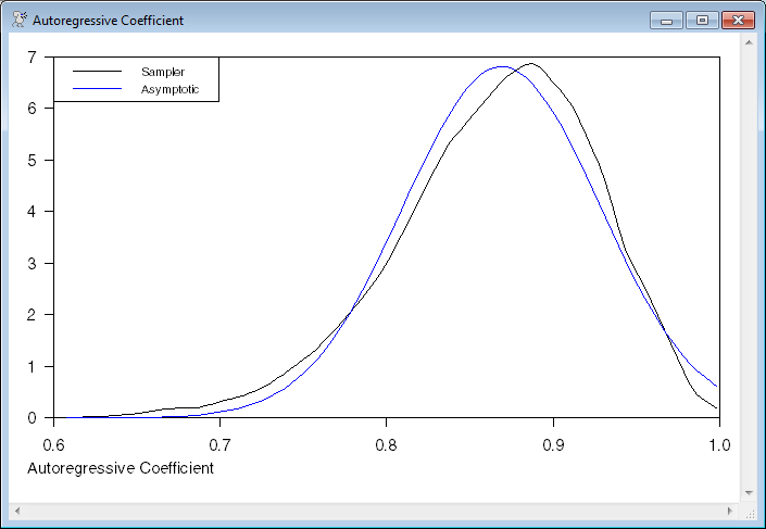
* This compares the empirical distribution from the sampler with the
* asymptotic distribution for the two ARMA coefficients.
*
set macoeff 1 ndraws = bgibbs(t)(3)
density(grid=automatic,maxgrid=100,smoothing=2.0) macoeff 1 ndraws xma fma
compute xxboxj=fxx*tr(fxx)
set fmabj 1 100 = exp(%logdensity(xxboxj(3,3),xma-bboxj(3)))
scatter(style=line,vmin=0.0,footer="Moving Average Coefficient",$
key=upleft,klabels=||"Sampler","Asymptotic"||) 2
# xma fma
# xma fmabj
*
set arcoeff 1 ndraws = bgibbs(t)(2)
density(grid=automatic,maxgrid=100,smoothing=2.0) arcoeff 1 ndraws xar far
compute xxboxj=fxx*tr(fxx)
set farbj 1 100 = exp(%logdensity(xxboxj(2,2),xar-bboxj(2)))
scatter(style=line,vmin=0.0,footer="Autoregressive Coefficient",$
key=upleft,klabels=||"Sampler","Asymptotic"||) 2
# xar far
# xar farbj

Output

Box-Jenkins - Estimation by ML Gauss-Newton

Convergence in 8 Iterations. Final criterion was 0.0000009 <= 0.0000100

Dependent Variable LOGPPI

Quarterly Data From 1960:02 To 2002:01

Usable Observations 168

Degrees of Freedom 165

Centered R^2 0.9996075

R-Bar^2 0.9996027

Uncentered R^2 0.9999929

Mean of Dependent Variable 4.0388032329

Std Error of Dependent Variable 0.5480971243

Standard Error of Estimate 0.0109244004

Sum of Squared Residuals 0.0196915164

Log Likelihood 521.6285

Durbin-Watson Statistic 1.9563

Q(36-2) 37.8097

Significance Level of Q 0.2994391

Variable Coeff Std Error T-Stat Signif

************************************************************************************

1. CONSTANT 0.007453020 0.003417646 2.18075 0.03061789

2. AR{1} 0.869012521 0.058641005 14.81920 0.00000000

3. MA{1} -0.452579062 0.103617498 -4.36779 0.00002210

Graphs