BIVARIATEHP.RPF

BIVARIATEHP.RPF provides an example of a bivariate Hodrick-Prescott (HP) filter. There's a common growth component for both series. Each series has its own intercept and loading on the growth component, that is, the model has

$\begin{array}{l}{y_{1,t}} = {a_1} + {g_1}{G_t} + {v_{1,t}} \\ {y_{2,t}} = {a_2} + {g_2}{G_t} + {v_{2,t}} \\ \end{array}$

where ${G_t}$ has a standard local trend state space model.

Because there are $n+1$ "intercepts" in the complete model (1 for each data series + 1 in the growth component), the series intercepts are constrained to sum to one. (This is accomplished by using the %perp of a vector of 1's premultiplying an $n-1$ vector of free coefficients). The "sv" matrix in the DLM gives the weighting scheme applied to the errors in the observables. If this is the identity matrix, the series get equal weights. Changing that to a non-identity will force G to fit better the series with the smaller value for SV.

Full Program

*
* Example of bivariate HP filter. This can be adapted to more than two
* variables, by changing the n=2 and redefining the YF vector.
*
open data oecdsample.rat
calendar(q) 1981
data(format=rats) 1981:1 2006:4 canexpgdpchs usaexpgdpch
*
set canrgdps   = log(canexpgdpchs)
set usargdps   = log(usaexpgdpch)
*
compute n=2
*
dec frml[vect] yf
frml yf = ||canrgdps,usargdps||
*
compute lambda=1600.0
*
* Standard local trend model for the common growth component
*
compute [rect] a=||1.0,1.0|0.0,1.0||
compute [symm] sw=%diag(||0.0,1.0/lambda||)
*
compute [symm] sv=%identity(n)
*
* Each series is modeled as y(i)=a(i)+gamma(i)*growth+v(i)
*
* Because there are n+1 "intercepts" in the complete model (1 for each
* data series + 1 in the growth component), the series intercepts are
* constrained to sum to one. (This is accomplished by using the %perp of
* a vector of 1's premultiplying an n-1 vector of free coefficients).
* The "sv" matrix in the DLM gives the weighting scheme applied to the
* errors in the observables. If this is the identity matrix, the series
* get equal weights.
*
dec vect gamma(n)
dec vect theta(n-1)
*
nonlin gamma theta
compute gamma=%const(1.0),theta=%const(0.0)
*
compute oneperp=%perp(%fill(1,n,1.0))
*
dec frml[rect] cf
frml cf = tr(gamma)~~%zeros(1,n)
*
* This has some convergence problems. The likelihood is extremely flat
* in the parameters, so almost identical trends can be generated many
* ways.
*
dlm(type=smooth,y=yf,mu=oneperp*theta,a=a,sw=sw,sv=sv,c=cf,$
presample=diffuse,var=concentrated,pmethod=simplex,piters=50,$
   method=bfgs) / xstates
*
set canf = %dot(%xrow(oneperp,1),theta)+%dot(%xcol(cf(t),1),xstates(t))
set usaf = %dot(%xrow(oneperp,2),theta)+%dot(%xcol(cf(t),2),xstates(t))
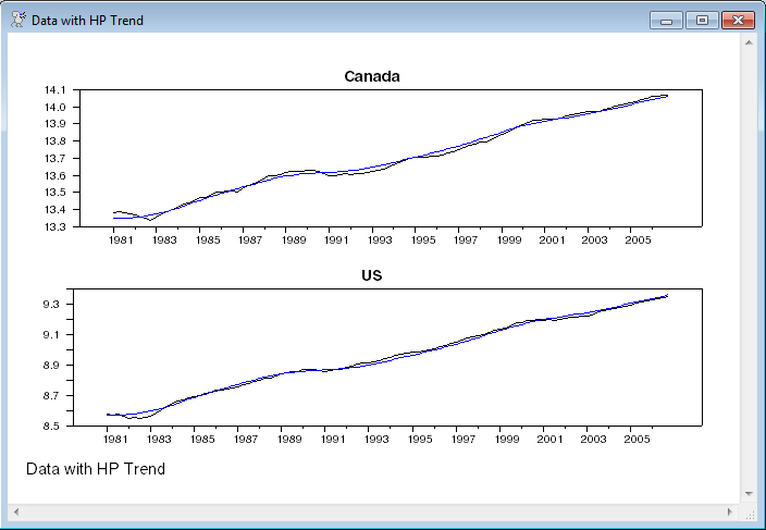
spgraph(vfields=2,footer="Data with HP Trend")
graph(header="Canada") 2
# canrgdps
# canf
graph(header="US") 2
# usargdps
# usaf
spgraph(done)
*
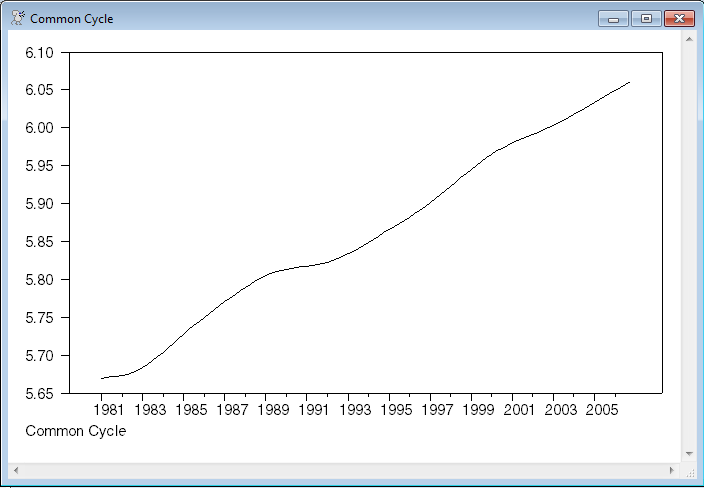
set cycle = xstates(t)(1)
graph(footer="Common Cycle")
# cycle

Output

This doesn't converge well. The likelihood is quite flat in the parameters.

DLM - Estimation by BFGS

NO CONVERGENCE IN 47 ITERATIONS

LAST CRITERION WAS 0.0000000

ESTIMATION POSSIBLY HAS STALLED OR MACHINE ROUNDOFF IS MAKING FURTHER PROGRESS DIFFICULT

TRY HIGHER SUBITERATIONS LIMIT, TIGHTER CVCRIT, DIFFERENT SETTING FOR EXACTLINE OR ALPHA ON NLPAR

RESTARTING ESTIMATION FROM LAST ESTIMATES OR DIFFERENT INITIAL GUESSES MIGHT ALSO WORK

Quarterly Data From 1981:01 To 2006:04

Usable Observations 104

Rank of Observables 206

Log Likelihood 535.9360

Concentrated Variance 2.6794e-004

Variable Coeff Std Error T-Stat Signif

************************************************************************************

1. GAMMA(1) 1.8364693441 0.0133547013 137.51482 0.00000000

2. GAMMA(2) 2.0289392716 0.0223115912 90.93656 0.00000000

3. THETA(1) 4.1489662672 0.1452974282 28.55499 0.00000000

Graphs