BRYBOSCHAN Procedure

@BRYBOSCHAN is an implementation of the Bry-Boschan business cycle dating algorithm. For quarterly data, it implements the Pagan-Harding(2002) version. This will typically be applied to the log of a deasonalized (but not detrended) macroeconomic series.

The Bry-Boschan algorithm is a complex multi-step process which (for monthly data)

1.Replaces "outliers" in the data (those too far from a preliminary trend-cycle).

2.Locates preliminary turning points by finding local maxima and minima of the adjusted trend-cycle.

3.Eliminates consecutive "peaks" and consecutive "troughs", by keeping the most extreme in a sequence.

4.Enforces a minimum cycle length (eliminating the less pronounced peak-trough combination to make that happen).

5.Does some further refinement to make sure "phases" aren't too short.

Note that it is not designed for (say) stock market data, which has a different definition for "bull" and "bear" markets based upon the magnitude of changes from previous highs and lows. Bry-Boschan does not have a requirement for how large a change is required to make a cycle, just minimum lengths and the requirement that peak follows trough and vice versa.

@BryBoschan( options ) series start end

Parameters

series	series to analyze
start, end	range of series to use. By default, the defined range of series.

Options

MA=width of centered MA used in final refinement [chosen based upon MCD criterion]

PRINT=[NONE]/FINAL/ALL

level of output desired

QUARTERLY/[NOQUARTERLY]

PEAK=(output) dummy variable series with 1's in the chosen peak entries

TROUGH=(output) dummy variable series with 1's in the chosen trough entries

UP=(output) 0-1 dummy series which is 1 from trough date + 1 until next peak date

DOWN=(output) 0-1 dummy series which is 1 from peak date + 1 until next trough date

Examples

These examples are based upon Mark Watson(1994). The monthly example is from the paper itself, while the quarterly uses the same data set, but is compacted to quarterly.

Monthly program

open data watsonaer.rat

cal(m) 1947

data(format=rats) 1947:1 1990:12 ip fycp fspcomr

log ip

@BryBoschan(print=all) ip 1947:1 1990:12

log fycp

@BryBoschan(print=final) fycp

log fspcomr

@BryBoschan(print=final,peak=peaks,trough=troughs) fspcomr

Quarterly program

open data watsonaer.rat

cal(q) 1947

data(format=rats) 1947:1 1990:4 ip fycp fspcomr

log ip

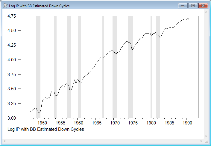
@BryBoschan(print=all,down=down,quarterly) ip 1947:1 1990:4

graph(shading=down,footer="Log IP with BB Estimated Down Cycles")

# ip

log fycp

@BryBoschan(print=final,quarterly) fycp

log fspcomr

@BryBoschan(print=final,quarterly) fspcomr

Sample output

This is the output from the quarterly log IP. The first is produced because of the PRINT=ALL, which shows a preliminary identification of turning points in step 2 above. Note that some of these (for instance 1951:2 and 1951:3) are eliminated in later steps (probably for having too short a "down" phase of just one quarter) and the minor "peak" at 1989:2 is dropped because it has no identifiable trough following it.

Step II

Peaks Troughs

1948:03 1949:04

1951:02 1951:03

1953:02 1954:02

1953:03 1956:03

1956:01 1958:02

1957:01 1961:01

1960:01 1967:02

1966:04 1970:04

1969:03 1974:01

1973:04 1975:02

1974:03 1979:03

1979:02 1980:03

1980:01 1982:04

1981:03 1986:02

1986:01

1989:02

Turning Points for Series IP

Peaks Peak-to-Peak Trough-to-Peak Troughs Trough-to-Trough Peak-to-Trough

1948:03 1949:04 5

1953:03 20 15 1954:02 18 3

1957:01 14 11 1958:02 16 5

1960:01 12 7 1961:01 11 4

1966:04 27 23 1967:02 25 2

1969:03 11 9 1970:04 14 5

1973:04 17 12 1975:02 18 6

1980:01 25 19 1980:03 21 2

1981:03 6 4 1982:04 9 5

1986:01 18 13

Graph

This is the quarterly version of IP, with the "down" cycle phases shaded.