COINTTST.RPF

COINTTST.RPF provides an example of tests for cointegration, demonstraing the procedures @EGTEST and @JOHMLE. It is adapted from Hamilton(1994). It examines whether the Purchasing Power Parity (PPP) restriction is a cointegrating vector for Italian and U.S. data:

$\log \,P_t - \log \,S_t - \log \,P_t^* $

where $P_t$ and $P_t^*$ are the price levels in the two countries and $S_t$ is the exchange rate. The raw data are a measure of the Italian price level (PC6IT), the U.S. price level (PZUNEW) and the exchange rate (EXRITL, as Italian lira per U.S. $).

cal(m) 1973:1

open data exdata.rat

data(format=rats) 1973:1 1989:10 pc6it pzunew exritl

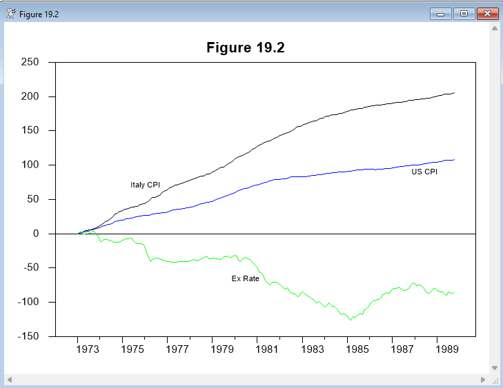
This transforms the data to 100*logs. The division by the value in 1973:1 normalizes the series to 1 in 1973:1 (which converts to a starting value of 0 when done in logs. This makes it easier to do graphs on a common scale and has no effect on any test statistics.

set italcpi = 100*log(pc6it/pc6it(1973:1))

set uscpi = 100*log(pzunew/pzunew(1973:1))

set exrat = -100*log(exritl/exritl(1973:1))

This does a graph of the three logged normalized series on a single graph.

graph(header="Figure 19.2",key=attached,klabel=||"Italy CPI","US CPI","Ex Rate"||) 3

# italcpi

# uscpi

# exrat

The first step is testing whether the series are I(1) with Dickey-Fuller tests (all three pass easily):

@dfunit(lags=12,trend) uscpi

@dfunit(lags=12,trend) italcpi

@dfunit(lags=12,trend) exrat

The test for PPP being a cointegrating relation is done with:

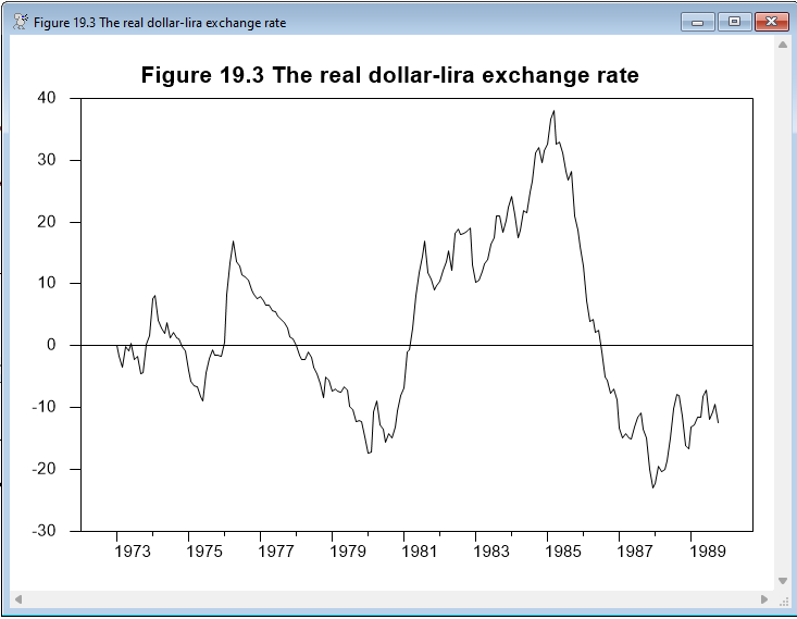
set ppp = uscpi-exrat-italcpi

graph(header="Figure 19.3 The real dollar-lira exchange rate")

# ppp

@dfunit(lags=12) ppp

If the variables are cointegrated and we have used the correct cointegrating vector, then this series should fail a unit root test (it should be a stationary series). As this ends up accepting the unit root, we reject the null hypothesis of cointegration–the deviations from PPP are not stationary (which seems clear from the graph of the PPP series).

Testing an Unknown Cointegrating Vector

The simplest testing procedure for cointegration with an unknown cointegrating vector is to apply a unit root test to the residuals from a regression involving the variables. This is the Engle-Granger test. Since the sum of squares of a non-stationary linear combination should be quite a bit higher than those for a stationary linear combination, we would expect that least squares would zero in on a stationary linear combination if it exists. Thus it’s even more important in this case to make sure the input variables are themselves I(1). Because the coefficients are now estimated, the critical values for the unit root test are different and get more negative the more variables we include in the cointegrating regression. There are two procedures for doing this: @EGTestResids takes as input the residuals from the cointegrating regression. @EGTest takes the set of variables and does the preliminary regression itself.

@EGTEST has most of the same options as @DFUNIT but because the number of endogenous variables isn’t fixed, they are input to the procedure using a supplementary card. Although it’s unlikely to be interesting in this case (for the reasons described above), the Engle-Granger test can be applied to the three series in the example with something like:

@egtest(lags=12)

# uscpi italcpi exrat

The output from this is the least squares regression (using the first listed variable as the dependent variable) followed by the unit root test with critical values appropriate to the 3 variable test. The null of a unit root means no cointegration, and we do not reject that, so it does not appear that there is cointegration among these three. (And also the coefficients don't seem be bear any resemblance to what we would expect if PPP holds).

Note that the test statistic will be slightly different (though almost never substantially different) if you rearrange the regressors to use a different series first (which will change the dependent variable in the least squares regression).

An alternative to the regression-based tests is the likelihood ratio approach, which is the basis for the CATS software. The likelihood approach allows for testing sequentially for the rank of cointegration from 0 (no cointegration, N separate stochastic trends) up to N, which would mean no unit roots. See the discussion in Hamilton or Juselius.

The procedure @JOHMLE does the basic Johansen likelihood ratio test. In our example:

@johmle(lags=6,det=constant)

# uscpi italcpi exrat

DET=CONSTANT is appropriate for this example because that means a constant in each equation outside the cointegrating vector, which allows for trends in the variables. From top to bottom, we reject ranks 0, 1 and 2. What does this mean? We reject all the restricted models in favor of the unrestricted VAR. That is often interpreted as meaning the VAR is "stationary". However, the eigenvalues of the test will always be between 0 and 1 regardless of the dynamic properties of the data. In particular, if the model had explosive roots, we would also reject rank=0 since the model in first differences can't adequately capture the explosive nature of the data. While the three series aren't explosive, there is likely some other structural change in this run of data which throws off the simple count of "roots".

Full Program

cal(m) 1973:1
open data exdata.rat
data(format=rats) 1973:1 1989:10 pc6it pzunew exritl
*
* Transform and normalize the data series
*
set italcpi = 100*log(pc6it/pc6it(1973:1))
set uscpi = 100*log(pzunew/pzunew(1973:1))
set exrat = -100*log(exritl/exritl(1973:1))
*
graph(header="Figure 19.2",key=attached,klabel=||"Italy CPI","US CPI","Ex Rate"||) 3
# italcpi
# uscpi
# exrat
*
* Dickey-Fuller tests on the variables
*
@dfunit(lags=12,trend) uscpi
@dfunit(lags=12,trend) italcpi
@dfunit(lags=12,trend) exrat
*
* Unit root tests on the hypothesized cointegrating vector
*
set ppp = uscpi-exrat-italcpi
graph(header="Figure 19.3 The real dollar-lira exchange rate")
# ppp
@dfunit(lags=12) ppp
*
* Engle-Granger test
* (Dickey-Fuller test with estimated cointegrating vector)
*
@egtest(lags=12)
# uscpi italcpi exrat
*
* Johansen maximum likelihood test
*
@johmle(lags=6,det=constant)
# uscpi italcpi exrat
*
* Using CATS (if you have it)
*
*@cats(lags=6,det=drift)
*# uscpi italcpi exrat

Output

Dickey-Fuller Unit Root Test, Series USCPI

Regression Run From 1974:02 to 1989:10

Observations 190

With intercept and trend

Using fixed lags 12

Sig Level Crit Value

1%(**) -4.00908

5%(*) -3.43435

10% -3.14084

T-Statistic -1.95467

Dickey-Fuller Unit Root Test, Series ITALCPI

Regression Run From 1974:02 to 1989:10

Observations 190

With intercept and trend

Using fixed lags 12

Sig Level Crit Value

1%(**) -4.00908

5%(*) -3.43435

10% -3.14084

T-Statistic -0.13196

Dickey-Fuller Unit Root Test, Series EXRAT

Regression Run From 1974:02 to 1989:10

Observations 190

With intercept and trend

Using fixed lags 12

Sig Level Crit Value

1%(**) -4.00908

5%(*) -3.43435

10% -3.14084

T-Statistic -1.58443

Dickey-Fuller Unit Root Test, Series PPP

Regression Run From 1974:02 to 1989:10

Observations 190

With intercept

Using fixed lags 12

Sig Level Crit Value

1%(**) -3.46588

5%(*) -2.87674

10% -2.57479

T-Statistic -2.03940

Linear Regression - Estimation by Least Squares

Dependent Variable USCPI

Monthly Data From 1973:01 To 1989:10

Usable Observations 202

Degrees of Freedom 199

Centered R^2 0.9944358

R-Bar^2 0.9943799

Uncentered R^2 0.9988561

Mean of Dependent Variable 63.896005070

Std Error of Dependent Variable 32.584534846

Standard Error of Estimate 2.442773037

Sum of Squared Residuals 1187.4608822

Regression F(2,199) 17782.7795

Significance Level of F 0.0000000

Log Likelihood -465.5274

Durbin-Watson Statistic 0.0277

Variable Coeff Std Error T-Stat Signif

************************************************************************************

1. ITALCPI 0.5300409655 0.0067083855 79.01170 0.00000000

2. EXRAT 0.0513484775 0.0120453693 4.26292 0.00003114

3. Constant 2.7123129580 0.3676954952 7.37652 0.00000000

Engle-Granger Cointegration Test

Null is no cointegration (residual has unit root)

Regression Run From 1974:02 to 1989:10

Observations 190

Using fixed lags 12

Constant in cointegrating vector

Critical Values from MacKinnon for 3 Variables

Test Statistic -2.73094

1%(**) -4.37196

5%(*) -3.78723

10% -3.48472

Likelihood Based Analysis of Cointegration

Variables: USCPI ITALCPI EXRAT

Estimated from 1973:07 to 1989:10

Data Points 196 Lags 6 with Constant

Unrestricted eigenvalues, -T log(1-lambda) and Trace Test

Roots Rank EigVal Lambda-max Trace Trace-95%

3 0 0.1058 21.9184 39.6824 29.3800

2 1 0.0650 13.1681 17.7641 15.3400

1 2 0.0232 4.5959 4.5959 3.8400

Cointegrating Vector for Largest Eigenvalue

USCPI ITALCPI EXRAT

-0.547461 0.314870 0.048427

Graphs