COPULA.RPF

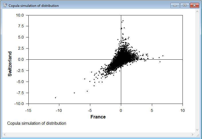
COPULA.RPF demonstrates use of a copula as an alternative to a multivariate GARCH model. A copula models a multivariate set of data by taking separate "marginal" models for the individual series (here AR(1) with t-distributed univariate GARCH errors) and uses one of a number of flexible functional forms for the joint distribution of standardized univariate results. This would be most similar to the parametric CC or DCC GARCH model, which also uses separate univariate GARCH models for the components. This does five different forms for the copulae, each of which needs a maximum likelihood estimate of one or two shape parameters. It does a simulation of the estimated joint distribution of the data using the last estimated copula model (the Gumbel EML), which shows that the data are more highly correlated when both are negative than otherwise (while a standard CC-GARCH model predicts similar clustering for both positive as with both negative).

Full Program

open data g10xrate.xls
data(format=xls,org=columns) 1 6237 usxjpn usxfra usxsui
*
compute nvar=2
*
set xfra = 100.0*log(usxfra/usxfra{1})
set xsui = 100.0*log(usxsui/usxsui{1})
*
* Use AR(1) models for the means
*
equation eqfra xfra
# constant xfra{1}
equation eqsui xsui
# constant xsui{1}
group mvar1 eqfra eqsui
*
* For copula, standardize with univariate student-t GARCH models with univariate
* AR(1) mean models.
*
garch(p=1,q=1,equation=eqfra,hseries=hfra,distrib=t)
*
* Standardized residuals
*
set zfra = %resids/sqrt(hfra)
*
* Empirical distribution of standardized residuals
*
order(ranks=rfra) zfra
set rfra = rfra/%nobs
*
* Marginal distribution given the estimated t distribution. fixt is to correct for
* the fact that GARCH models model the variance of the distribution, not the
* variance of the underlying Normal.
*
compute nufra=%shape
compute fixt=(nufra-2)/nufra
set mfra = %tcdf(zfra/sqrt(fixt),nufra)
*
garch(p=1,q=1,equation=eqsui,hseries=hsui)
set zsui = %resids/sqrt(hsui)
order(ranks=rsui) zsui
set rsui = rsui/%nobs
compute nusui=%shape
compute fixt=(nusui-2)/nusui
set msui = %tcdf(zsui/sqrt(fixt),nusui)
*
* Gaussian copula estimation
*
* Parameterize subdiagonal
*
dec packed[real] qsub(nvar-1,nvar-1)
compute qsub=%const(0.0)
*
function %subtocorr sub
type packed sub
type symm   %subtocorr
local integer i j
*
dim %subtocorr(%rows(sub)+1,%rows(sub)+1)
ewise %subtocorr(i,j)=%if(i==j,1.0,sub(i-1,j))
end
*
* This should be almost identical to a CC model with Normal residuals. (The
* difference is because the CC model does joint estimates of all parameters).
*
frml gcopula = %logdensity(%subtocorr(qsub),||zfra,zsui||)
nonlin qsub
maximize gcopula
*
* Student t copula estimation
*
compute nu=10.0
*
frml tcopula = %logtdensitystd(%subtocorr(qsub),||zfra,zsui||,nu)
nonlin qsub nu
maximize tcopula
*
* CML estimation
*
* Gaussian copula CML estimator
*
nonlin qsub
frml gcopula_cml = %logdensity(%subtocorr(qsub),||%invnormal(rfra),%invnormal(rsui)||)
maximize gcopula
*
* Bivariate Gumbel CML estimator
*
compute theta=1.0
nonlin theta
frml gumbel_cml = -(theta+1)*(log(rfra)+log(rsui))-(1.0/theta+2)*log(rfra^-theta+rsui^-theta)
maximize gumbel_cml
*
* Gumbel estimator using t marginals with degrees of freedom from GARCH model
*
frml gumbel_eml = -(theta+1)*(log(mfra)+log(msui))-(1.0/theta+2)*log(mfra^-theta+msui^-theta)
maximize gumbel_eml
*
compute ndraws=10000
clear(length=ndraws) xxfra xxsui
do draw=1,ndraws
   compute u=%uniform(0.0,1.0)
   compute p=%uniform(0.0,1.0)
   compute v=((p^-(theta/(theta+1))-1)*u^(-theta)+1)^(-1.0/theta)
   *
   * Back-transform using the t-distribution
   *
   compute dfra=%invtcdf(u,nufra)
   compute dsui=%invtcdf(v,nufra)
   *
   * Back transform using the variances at the final entry.
   *
   compute dfra=dfra*sqrt(hfra(6237)*(nufra-2)/nufra)
   compute dsui=dsui*sqrt(hsui(6237)*(nusui-2)/nusui)
   compute xxfra(draw)=dfra
   compute xxsui(draw)=dsui
end do draw
*
* The draws are much more correlated in the left tail than the right tail
*
scatter(hlabel="France",vlabel="Switzerland",footer="Copula simulation of distribution")
# xxfra xxsui

Output

GARCH Model - Estimation by BFGS

Convergence in 88 Iterations. Final criterion was 0.0000018 <= 0.0000100

Dependent Variable XFRA

Usable Observations 6235

Log Likelihood -5157.5075

Variable Coeff Std Error T-Stat Signif

************************************************************************************

1. Constant -0.000238111 0.004414505 -0.05394 0.95698427

2. XFRA{1} 0.012474767 0.011404957 1.09380 0.27404172

3. C 0.000633580 0.000378790 1.67264 0.09439764

4. A 0.117800580 0.013220939 8.91015 0.00000000

5. B 0.904031905 0.009349362 96.69450 0.00000000

6. Shape 3.968679780 0.215983415 18.37493 0.00000000

GARCH Model - Estimation by BFGS

Convergence in 26 Iterations. Final criterion was 0.0000015 <= 0.0000100

Dependent Variable XSUI

Usable Observations 6235

Log Likelihood -6682.4241

Variable Coeff Std Error T-Stat Signif

************************************************************************************

1. Constant 0.0032808765 0.0080099138 0.40960 0.68209795

2. XSUI{1} 0.0307519315 0.0144726122 2.12484 0.03360028

3. C 0.0109495148 0.0019932273 5.49336 0.00000004

4. A 0.0962372038 0.0086045400 11.18447 0.00000000

5. B 0.8896242340 0.0099611213 89.30965 0.00000000

MAXIMIZE - Estimation by BFGS

Convergence in 9 Iterations. Final criterion was 0.0000035 <= 0.0000100

Usable Observations 6235

Skipped/Missing (from 6237) 2

Function Value -14458.7411

Variable Coeff Std Error T-Stat Signif

************************************************************************************

1. QSUB(1,1) 0.8032886995 0.0035059100 229.12417 0.00000000

MAXIMIZE - Estimation by BFGS

Convergence in 10 Iterations. Final criterion was 0.0000028 <= 0.0000100

Usable Observations 6235

Skipped/Missing (from 6237) 2

Function Value -12975.3291

Variable Coeff Std Error T-Stat Signif

************************************************************************************

1. QSUB(1,1) 0.8436714418 0.0037741950 223.53679 0.00000000

2. NU 4.0311334565 0.0948347631 42.50692 0.00000000

MAXIMIZE - Estimation by BFGS

Convergence in 6 Iterations. Final criterion was 0.0000079 <= 0.0000100

Usable Observations 6235

Skipped/Missing (from 6237) 2

Function Value -14458.7411

Variable Coeff Std Error T-Stat Signif

************************************************************************************

1. QSUB(1,1) 0.8032887282 0.0034977556 229.65834 0.00000000

MAXIMIZE - Estimation by BFGS

Convergence in 7 Iterations. Final criterion was 0.0000004 <= 0.0000100

Usable Observations 6235

Skipped/Missing (from 6237) 2

Function Value -6688.9865

Variable Coeff Std Error T-Stat Signif

************************************************************************************

1. THETA 1.7119669392 0.0220253727 77.72704 0.00000000

MAXIMIZE - Estimation by BFGS

Convergence in 4 Iterations. Final criterion was 0.0000000 <= 0.0000100

Usable Observations 6235

Skipped/Missing (from 6237) 2

Function Value -6674.7088

Variable Coeff Std Error T-Stat Signif

************************************************************************************

1. THETA 1.6939348950 0.0216443777 78.26212 0.00000000

Graphs