DLMEXAM2.RPF

DLMEXAM2.RPF is an example of Kalman filtering and out-of-sample forecasts. This uses the model for Nile river flow data common to the four simple DLM examples.

The out-of-sample forecasts (for 10 years out-of-sample) can be done simply by running the Kalman filter (TYPE=FILTER) from the start of the sample to the end of the forecast period. Once there is no longer data in the Y series, the Kalman filter just does the prediction step and not the correction step.

Since the data end in 1970:1, the end of forecast period is 1980:1. This uses several other options for output. The YHAT option gives the predictions for Y and SVHAT gives the forecast variance.

dlm(a=1.0,c=1.0,sv=15099.0,sw=1469.1,y=nile,presample=diffuse,$

type=filter,yhat=yhat,svhat=svhat) * 1980:1

This pulls out the out-of-sample forecasts (into FORECAST) and the corresponding standard errors (into STDERR), and LOWER and UPPER as bounds for 50% confidence intervals.

set forecast 1971:1 1980:1 = %scalar(yhat)

set stderr 1971:1 1980:1 = sqrt(%scalar(svhat))

set lower 1971:1 1980:1 = forecast+%invnormal(.25)*stderr

set upper 1971:1 1980:1 = forecast+%invnormal(.75)*stderr

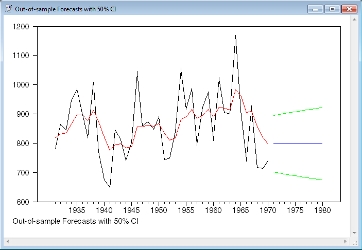
The actual data (for part of the data set), forecasts and confidence interval are graphed.

Full Program

open data nile.dat
calendar 1871
data(format=free,org=columns,skips=1) 1871:1 1970:1 nile
*
* Kalman filter through the data period, and then out 10 years beyond.
*
dlm(a=1.0,c=1.0,sv=15099.0,sw=1469.1,y=nile,presample=diffuse,$
type=filter,yhat=yhat,svhat=svhat) * 1980:1 xstate
*
set filtered *      1970:1 = %scalar(xstate)
set forecast 1971:1 1980:1 = %scalar(yhat)
set stderr   1971:1 1980:1 = sqrt(%scalar(svhat))
*
set lower 1971:1 1980:1 = forecast+%invnormal(.25)*stderr
set upper 1971:1 1980:1 = forecast+%invnormal(.75)*stderr
graph(footer="Out-of-sample Forecasts with 50% CI") 5
# nile     1931:1 1970:1
# filtered 1931:1 1970:1 4
# forecast / 2
# lower    / 3
# upper    / 3

Graph