DSGEKPR.RPF

DSGEKPR.RPF is an example of solution of a non-linear DSGE model. This demonstrates the DSGE instruction and the @DLMIRF procedure.

Watson (1993) analyzes a special case of the model below (with some minor renaming of variables) whose equilibrium is described by the following equations:

\begin{equation} \frac{\theta }{{1 - N_t }} = C_t^{ - \eta } \alpha \frac{{Y_t }}{{N_t }} \end{equation}

\begin{equation} 1 = \beta \gamma ^{1 - \eta } E_t R_{t + 1} \left( {{{C_t } \mathord{\left/ {\vphantom {{C_t } {C_{t + 1} }}} \right. } {C_{t + 1} }}} \right)^\eta \end{equation}

\begin{equation} \gamma R_t = \left( {1 - \alpha } \right)\frac{{Y_t }}{{K_{t - 1} }} + 1 - \delta \end{equation}

\begin{equation} C_t + I_t = Y_t \end{equation}

\begin{equation} \gamma K_t = I_t + \left( {1 - \delta } \right)K_{t - 1} \end{equation}

\begin{equation} Y_t = Z_t K_{t - 1}^{1 - \alpha } N_t^\alpha \end{equation}

\begin{equation} \log Z_t = \left( {1 - \rho } \right)\log \left( {\bar Z} \right) + \rho \log \left( {Z_{t - 1} } \right) + \varepsilon _t \label{eq:dsgekpr_eq7} \end{equation}

There is only one exogenous shock in this model (equation \eqref{eq:dsgekpr_eq7}—the technology shock). This is a non-linear model, which will be analyzed using a log-linearization. Because $N$ (labor force participation rate) can’t take the value 1, we can’t use the default initial guess values for all variables, so the initial values parameters are used for some. SOLVEBY=SVD is included to deal with the unit root in the technology shock.

This is the King-Plosser-Rebelo(1988) model, hence the name of the program. However, the date conventions for capital are those recommended by Uhlig and Sims, rather than KPR's.

open data watson_jpe.rat

calendar(q) 1948:1

data(format=rats) 1948:1 1988:4 y c invst h

Several of the series used in the model are unobservable and so aren’t in the data set (which is never actually used in this example). They’re included in a DECLARE SERIES instruction so they can be used in defining the equations.

declare series n r z k

declare real theta eta alpha beta gamma delta psi

These are the calibration values used by Watson.

compute eta=1.0 Log utility

compute alpha=.58 Labor’s share

compute nbar=.2 Steady state level of hours

compute gamma=1.004 Rate of technological progress

compute delta=.025 Depreciation rate for capital (quarterly)

compute rq=.065/4 Quarterly steady state interest rate

compute rho=1.00 AR coefficient in technical change

compute lrstd=.01 Long-run standard deviation of output

compute zbar=1.0 Mean of technology process

compute theta=3.29 Preference parameter for leisure

compute beta=gamma/(1+rq)

Define the equations. F7 is the only one with a shock attached. F2 is the only one with an expectational term (for future $C$ and future $R$).

frml(identity) f1 = theta/(1-n)-c^(-eta)*alpha*y/n

frml(identity) f2 = 1-beta*gamma^(1-eta)*c/c{-1}*r{-1}

frml(identity) f3 = gamma*r-(1-alpha)*y/k{1}-1+delta

frml(identity) f4 = c+invst-y

frml(identity) f5 = gamma*k-invst-(1-delta)*k{1}

frml(identity) f6 = y-z*k{1}^(1-alpha)*n^alpha

frml f7 = log(z)-(1-rho)*log(zbar)-rho*log(z{1})

group swmodel f1 f2 f3 f4 f5 f6 f7

Solve the model to state-space form, overriding several settings for the guess values.

dsge(model=swmodel,expand=loglinear,a=a,f=f,solveby=svd) $

y c<<0.5 invst<<0.5 n<<nbar r<<1+rq k z

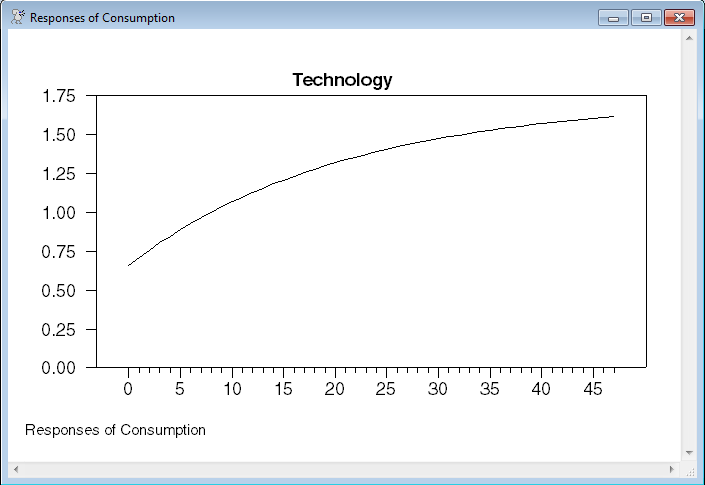
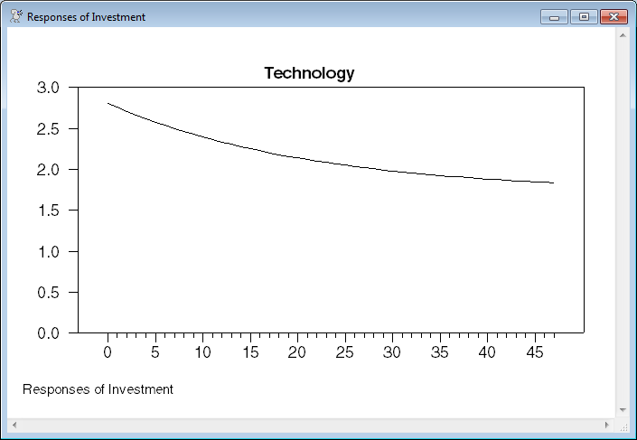
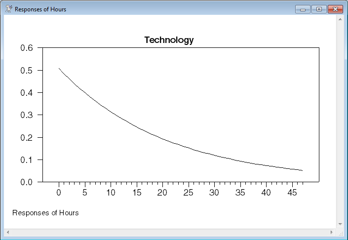
Graph the impulse responses using the state-space matrices. The state-space model will have more than four states, but by limiting the VARIABLES option, you only see the four main ones, and not R, K, Z and any augmenting states.

@dlmirf(a=a,f=f,graph=byvar,shocks=||"Technology"||,$

variables=||"Output","Consumption","Investment","Hours"||)

Full Program

*
* Replication program for Watson (1993), "Measures of Fit for Calibrated
* Models", J. of Political Economy, vol 101, pp 1011-1041. This uses the
* model from King, Plosser and Rebelo, but with the date conventions
* used by Uhlig and Sims, rather than KPR's.
*
* Get data. Income, consumption and investment are log real per capita
* values.
*
open data watson_jpe.rat
cal(q) 1948
data(format=rats) 1948:1 1988:4 y c invst h
*
* theta/(1-N(t))=C(t)^(-eta)alpha*Y(t)/N(t)
* 1=(beta-star)*Et[(C(t)/C(t+1))^eta R(t+1)], where beta-star=beta*gamma^(1-eta)
* gamma R(t)=(1-alpha)*Y(t)/K(t-1)+1-delta
*
* with
*
* C(t)+I(t)=Y(t)
* gamma K(t)=I(t)+(1-delta)*K(t-1)
* Y(t)=Z(t)*K(t-1)^(1-alpha)*N(t)^alpha
* log Z(t)=(1-psi)*log(Z-bar)+psi*log(Z(t-1))+eps(t)
*
* Several of the series used in the model are unobservable and so aren’t
* in the data set. (The data aren't used in this short example). They’re
* included in a DECLARE SERIES instruction so they can be used in
* defining the equations.
*
declare series n r z k
*
declare real theta eta alpha beta gamma delta psi
*
* Calibration values used by Watson
*
compute eta=1.0      ;* Log utility
compute alpha=.58    ;* Labor's share
compute nbar=.2      ;* Steady state level of hours (used in place of "A" in utility function)
compute gamma=1.004 ;* Rate of technological progress
compute delta=.025   ;* Depreciation rate for capital (quarterly)
compute rq=.065/4    ;* Quarterly steady state interest rate
compute rho=1.00     ;* AR coefficient in technical change
compute lrstd=.01    ;* Long-run standard deviation of output
compute zbar=1.0     ;* Mean of technology process
compute theta=3.29   ;* Preference parameter for leisure

compute beta=gamma/(1+rq)
compute sigma=lrstd*alpha
*
* Define the equations. F7 is the only one with a shock attached. F2 is
* the only one with an expectational term (for future C).
*
frml(identity) f1 = theta/(1-n)-c^(-eta)*alpha*y/n
frml(identity) f2 = 1-beta*gamma^(1-eta)*c/c{-1}*r{-1}
frml(identity) f3 = gamma*r-(1-alpha)*y/k{1}-1+delta
frml(identity) f4 = c+invst-y
frml(identity) f5 = gamma*k-invst-(1-delta)*k{1}
frml(identity) f6 = y-z*k{1}^(1-alpha)*n^alpha
frml           f7 = log(z)-(1-rho)*log(zbar)-rho*log(z{1})
*
group swmodel f1 f2 f3 f4 f5 f6 f7
*
* Solve the model to state-space form, overriding several settings for
* the guess values.
*
dsge(model=swmodel,expand=loglinear,a=a,f=f,solveby=svd) $
   y c<<0.5 invst<<0.5 n<<nbar r<<1+rq k z
*
* Graph the impulse responses using the state-space matrices. The
* state-space model will have more than four states, but by limiting the
* VARIABLES option, you only see the four main ones, and not R, K, Z and
* any augmenting states.
*
@dlmirf(a=a,f=f,page=byvar,shocks=||"Technology"||,$
   variables=||"Output","Consumption","Investment","Hours"||)

Graphs