GARCHMVDCCGIBBS.RPF

GARCHMVDCCGIBBS.RPF is an example of Gibbs sampling with DCC GARCH model.

Full Program

open data g10xrate.xls
data(format=xls,org=columns) 1 6237 usxjpn usxfra usxsui
*
set xjpn = 100.0*log(usxjpn/usxjpn{1})
set xfra = 100.0*log(usxfra/usxfra{1})
set xsui = 100.0*log(usxsui/usxsui{1})
compute n=3
dec vect[strings] vlabels(n)
compute vlabels=||"Japan","France","Switzerland"||
***********************************************************************
garch(p=1,q=1,mv=dcc,rvectors=rv,hmatrices=h) / xjpn xfra xsui
compute gstart=%regstart(),gend=%regend()
*
* Proposal density for the increment in independence chain MH is based
* upon the covariance matrix from the GARCH estimates. This is a
* multivariate t with <<nuxx>> degrees of freedom. The scale on FXX and
* the value for NUXX may need to be adjusted in different applications
* to get a reasonable acceptance rate.
*
compute fxx=.5*%decomp(%xx)
compute nuxx=10.0
*
* Start at the ML estimates
*
compute logplast=%logl
compute blast=%beta
compute accept=0
*
compute nburn=1000,nkeep=1000
*
* This keeps track of the DCC correlations estimates. This is a
* complicated structure since we have, for each draw, one full series
* for each off-diagonal. (For simplicity, this is also saving the
* diagonals, which are, of course, 1's). With a bigger model (longer
* time series or more variables) or more draws, you could run into
* memory issues.
*
dec symm[series[vect]] dcccorr(n,n)
do i=1,n
   do j=1,i
      gset dcccorr(i,j) gstart gend = %zeros(nkeep,1)
   end do j
end do i
*
dec series[symm] hlast
gset hlast gstart gend = h
*
infobox(action=define,progress,lower=-nburn,upper=nkeep) "Independence M-H"
do draw=-nburn,nkeep
   compute btest=blast+%ranmvt(fxx,nuxx)
   *
   * Evaluate the GARCH model at the proposal
   *
   garch(p=1,q=1,mv=dcc,initial=btest,method=evaluate,rvectors=rv,hmatrices=htest) / xjpn xfra xsui
   compute logptest=%logl
   *
   * Carry out the Metropolis test
   *
   compute alpha=exp(logptest-logplast)
   if alpha>1.0.or.%uniform(0.0,1.0)<alpha {
      compute accept=accept+1
      compute blast =btest
      compute logplast=logptest
      gset hlast gstart gend = htest
   }

   infobox(current=draw) %strval(100.0*accept/(draw+nburn+1),"##.##")
   if draw>0 {
      do i=1,n
         do j=1,i
            do t=gstart,gend
               compute dcccorr(i,j)(t)(draw)=%cvtocorr(hlast(t))(i,j)
            end do t
         end do j
      end do i
   }
end do draw
infobox(action=remove)
*
dec vect xcorr(nkeep)
dec symm[series] lower(n,n) upper(n,n) median(n,n)
clear(zeros) lower upper median
*
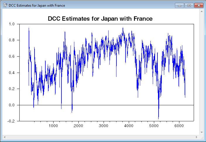
* Generate the median and 90% confidence band for the DCC correlations.
* For this data set, the period to period movement is large enough
* relative to the spread that the three lines basically end up on top of
* each other. If you graph over a shorter period, you can see at least
* some spread between the upper and lower bounds.
*
do j=2,n
   do k=1,j-1
      do t=gstart,gend
         ewise xcorr(i)=dcccorr(j,k)(t)(i)
         compute frac=%fractiles(xcorr,||.05,.50,.95||)
         compute lower(j,k)(t)=frac(1)
         compute upper(j,k)(t)=frac(3)
         compute median(j,k)(t)=frac(2)
      end do tme
      graph(header="DCC Estimates for "+vlabels(k)+" with "+vlabels(j)) 3
      # median(j,k) gstart gend
      # lower(j,k) gstart gend 2
      # upper(j,k) gstart gend 2
   end do k
end do j

Output

MV-DCC GARCH - Estimation by BFGS

Convergence in 40 Iterations. Final criterion was 0.0000080 <= 0.0000100

Usable Observations 6236

Log Likelihood -11814.4403

Variable Coeff Std Error T-Stat Signif

************************************************************************************

1. Mean(XJPN) 0.003987923 0.006009027 0.66366 0.50691089

2. Mean(XFRA) -0.003132340 0.006238983 -0.50206 0.61562576

3. Mean(XSUI) -0.003069840 0.007698257 -0.39877 0.69006207

4. C(1) 0.008499197 0.001141242 7.44732 0.00000000

5. C(2) 0.012485965 0.001377298 9.06555 0.00000000

6. C(3) 0.016566678 0.001823971 9.08276 0.00000000

7. A(1) 0.151663636 0.009063915 16.73268 0.00000000

8. A(2) 0.138383290 0.007750557 17.85463 0.00000000

9. A(3) 0.123692432 0.007406780 16.69989 0.00000000

10. B(1) 0.852004681 0.008025825 106.15790 0.00000000

11. B(2) 0.848526128 0.007936097 106.91982 0.00000000

12. B(3) 0.858001040 0.007867699 109.05362 0.00000000

13. DCC(A) 0.053230483 0.003249015 16.38358 0.00000000

14. DCC(A) 0.939072178 0.003941594 238.24678 0.00000000

Graphs

For this data set, the period to period movement is large enough relative to the spread that the three lines basically end up on top of each other. If you graph over a shorter period, you can see at least some spread between the upper and lower bounds.

This is one of three graphs generated by the program.