GCONTOUR Instruction

GCONTOUR( options ) hfield vfield

Generates a high-resolution contour plot.

Parameters

hfield, vfield

horizontal and vertical field (only with SPGRAPH with HFIELDS and/or VFIELDS options). You can now use the COL and ROW options instead.

Options Specific to GCONTOUR

The following is a list of the options for GCONTOUR. Many of these are identical to options on SCATTER, while some are unique to GCONTOUR. The options specific to GCONTOUR are described in detail here. See SCATTER for details on the other options.

X=VECTOR of X grid values [required]

Y=VECTOR of Y grid values [required]

F=RECTANGULAR array supplying function values [required]

Use the X option to supply a vector with the grid values for the x-axis, and the Y option to supply a vector with grid values for the y-axis. Use the F option to supply a RECTANGULAR array with dimensions , containing the function values for each x,y grid point. For example, F(1,2) should contain the function value associated with the grid point given by X(1),Y(2). X and Y are usually created using the %SEQA function or EWISE instruction. The F array is usually set using EWISE.

NUMBER=number of contour lines [30]

CONTOURS=VECTOR of specific “f” values

You can use CONTOURS to supply a VECTOR containing the specific function values at which you want contour lines to be plotted. Otherwise, RATS will draw the number of contour lines specified by the NUMBER option, with the contour values chosen to provide a roughly equal distance between each value.

Options Common to GCONTOUR and SCATTER

[AXIS]/NOAXIS	Draw horizontal axis if Y=0 is within graph bounds
COL=column number	Column position in an SPGRAPH array
EXTEND=NONE/VERTICAL/HORIZONTAL/[BOTH]	Extend grid lines across graph
FOOTER=footer label	Adds a footer label below graph
FRAME=[FULL]/HALF/NONE/BOTTOM	Controls frame around the graph
HEADER=string	Adds a header to the top of the graph
HEIGHT=value	Sets the height of the graph
HGRID=VECTOR for grid	Sets grid for horizontal axis
HLABEL=scale label	Adds a label to the horizontal axis
HLOG=base for log scale	Base for log scale graphs
HMAX=value for right	Sets the maximum x-axis value
HMIN=value for left	Sets the minimum x-axis value
HPICTURE="picture code"	Picture code for formatting x-axis label numbers
HSCALE=[LOWER]/UPPER/BOTH/NONE	Placement of x-axis scale
HSHADE=RECTANGULAR for shading zones	Shading zones for the y-axis
HTICKS=tick limit	Maximum number of tick marks on x-axis
LINES=RECTANGULAR with slope/intercept	Draw lines given slope/intercept
ROW=row number	Row position in an SPGRAPH array
SUBHEAD=string	Subheader string for graph
VGRID=VECTOR for grid	Sets grid for vertical axis
VLABEL=label	Label for the vertical axis
VLOG=base for log scale	Selects a log scale for y-axis
VMAX=value for upper	Sets maximum y-axis value
VMIN=value for lower	Sets minimum y-axis value
VPICTURE="picture code"	Picture code for formatting y-axis label numbers
VSCALE=[LEFT]/RIGHT/BOTH/NONE	Placement of vertical scale
VSHADE=RECTANGULAR for shading zones	Shading zones for the y-axis
VTICKS=number	Maximum number of ticks on the y-axis
WIDTH=value	Sets the width of the graph
WINDOW=string	Title for graph window
XLABELS=VECT[STRING]	Strings for labeling x-axis

Example

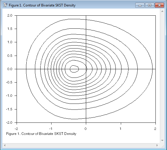
This creates a contour graph of the multivariate skew-t density, over the range from -2 to 2 in both the x and y dimensions. The %LOGMVSKEWT function returns the log density, so this is exp'ed to give the density itself. This uses an input set of contours, which generally requires some trial and error to get a good appearance.

* Reference: Bauwens & Laurent(2005), "A New Class of Multivariate Skew

* Densities, With Application to Generalized Autoregressive Conditional

* Heteroscedasticity Models," JBES, vol 23, pp 346-354.

source logmvskewt.src

@gridseries(from=-2.0,to=2.0,n=50) z1grid

@gridseries(from=-2.0,to=2.0,n=50) z2grid

dec rect f(51,51)

ewise f(i,j)=exp(%logmvskewt(||z1grid(j),z2grid(i)||,||1.0,1.3||,6.0))

dec vect contours(12)

ewise contours(i)=.02*i

gcontour(footer="Figure 1. Contour of Bivariate SKST Density",f=f,x=z2grid,y=z1grid,number=12,contours=contours)