GIBBSPROBITDYNAMIC.RPF

GIBBSPROBITDYNAMIC.RPF shows how to get a Gibbs sampling estimate of a dynamic "probit" model, where the latent index follows an AR(1) equation:

$y_t^* = \alpha + \rho y_{t - 1}^* + {\varepsilon _t},{\text{ with }}{\varepsilon _t}\sim N\left( {0,1} \right){\rm{ }}i.i.d.$

This uses the typical Gibbs sampling technique of drawing the continuous latent variable given the observable 0-1's, but, because of the dynamic process for the latent variable, you can't just draw those independently. Instead, the YSTAR are done one-at-a-time given the values of the YSTAR at all other data points.

Full Program

cal(q) 1960
@nbercycles(up=expansion) 1960:1 2009:4
*
* Start with ystar of +/-1
*
set ystar = %if(expansion,1.0,-1.0)
*
* Start the sampler at the OLS estimates, given the starting ystars
*
linreg ystar
# constant ystar{1}
compute rho=%beta(2),alpha=%beta(1)
*
* Set up state space model for ystar
*
frml af = rho
frml zf = alpha
*
* (diffuse) prior for coefficients
*
compute bprior=%zeros(2,1)
compute hprior=%zeros(2,2)
*
compute nburn=1000
compute ndraws=1000
*
dec series[vect] bgibbs
gset bgibbs 1 ndraws = %zeros(2,1)
set ystarhat = 0.0
*
infobox(action=define,progress,lower=-nburn,upper=ndraws) "Gibbs Sampler: Dynamic Probit"
do draw=-nburn,ndraws
   infobox(current=draw)
   *
   * Draw ystar(time) given all other ystar's. This is done by Gibbs
   * sampling on
   *
   * ystar(t)=alpha+rho*ystar(t-1)+eps(t) (state equation)
   * ystar(t)=ystar(t)+0 if t<>time        (measurement equation)
   *
   * Kalman smoothing gives the conditional mean and variance for
   * ystar(time).
   *
   do time=1960:1,2009:4
      dlm(y=%if(t==time,%na,ystar),a=af,z=zf,c=1.0,$
         sw=1.0,presample=ergodic,type=smooth) 1960:1 2009:4 xstates vstates
      compute cmean=%scalar(xstates(time)),cstddev=sqrt(%scalar(vstates(time)))
      *
      * Given the conditional mean and the observed value for the 0-1
      * variable, draw a truncated Normal for ystar.
      *
      compute ystar(time)=%if(expansion(time),%rantruncate(cmean,cstddev,0.0,%na),$
                                              %rantruncate(cmean,cstddev,%na,0.0))
   end do time
   *
   * Draw coefficients from the index equation given ystars
   *
   cmom
   # constant ystar{1} ystar
   compute bdraw=%ranmvpostcmom(%cmom,1.0,hprior,bprior)
   compute alpha=bdraw(1),rho=bdraw(2)
   *
   * After burn-in, save draws and add in the current estimate for YSTAR.
   *
   if draw>0 {
      compute bgibbs(draw)=bdraw
      set ystarhat = ystarhat+ystar
   }
end do draw
infobox(action=remove)
*
@mcmcpostproc(ndraws=ndraws,mean=bmean,stderrs=bstderrs,cd=bcd) bgibbs
*
report(action=define)
report(atrow=1,atcol=1,span) "MCMC Estimates for Dynamic Probit Model"
report(atrow=2,atcol=1) "Constant" bmean(1) bstderrs(1)
report(atrow=3,atcol=1) "YSTAR{1}" bmean(2) bstderrs(2)
report(action=format,picture="*.###")
report(action=show)
*
set ystarhat = ystarhat/ndraws
*
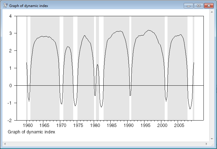
* Graph the (average across draws of the) dynamic index. Note that this is a
* "smoothed" estimate, as it uses the information from the full data set.
*
graph(shading=expansion,footer="Graph of dynamic index")
# ystarhat

Output

The MCMC estimates and the graph depend upon random numbers and so will not be exactly reproducible.

Linear Regression - Estimation by Least Squares

Dependent Variable YSTAR

Quarterly Data From 1960:02 To 2009:04

Usable Observations 199

Degrees of Freedom 197

Centered R^2 0.4705906

R-Bar^2 0.4679032

Uncentered R^2 0.7288851

Mean of Dependent Variable 0.6984924623

Std Error of Dependent Variable 0.7174222505

Standard Error of Estimate 0.5233233986

Sum of Squared Residuals 53.951873767

Regression F(1,197) 175.1128

Significance Level of F 0.0000000

Log Likelihood -152.5001

Durbin-Watson Statistic 1.7445

Variable Coeff Std Error T-Stat Signif

************************************************************************************

1. Constant 0.2193293886 0.0518397282 4.23091 0.00003564

2. YSTAR{1} 0.6859960552 0.0518397282 13.23302 0.00000000

MCMC Estimates for Dynamic Probit Model

Constant 0.353 0.124

YSTAR{1} 0.804 0.070

Graph