MIXTURE.RPF

MIXTURE.RPF is an example of a mixture model (not-Markovian) demonstrating the different estimation strategies. Note that this model has a "labeling" problem when you estimate by MCMC, as the attempt to define the regimes as "high" and "low" don't really work.

Full Program

open data ger4ind.prn
calendar(q) 1961
data(format=prn,org=columns) 1961:1 1986:4 ipgrowth
set x = 100.0*ipgrowth
*
* We'll use a two lag AR which will fully switch between regimes. In
* practice, this is probably too "loose" a model; there are almost
* certainly many modes for the likelihood function, since AR(2)'s can
* model many types of behavior.
*
equation xeq x
# constant x{1 to 2}
*
dec vect[vect] phi(2)
nonlin(parmset=regparms) phi sigsq
nonlin(parmset=msparms) p
*
* Set up guess values. The coefficient vectors are separated by giving
* the first a larger intercept.
*
linreg(equation=xeq)
compute rstart=%regstart(),rend=%regend()
compute phi(1)=%beta
compute phi(2)=%beta
compute phi(1)(1)+=sqrt(%seesq)
compute phi(2)(1)-=sqrt(%seesq)
compute sigsq=%seesq
*
* Save the guess values so we can use them when demonstrating different
* techniques. (This step isn't generally necessary).
*
compute guesses=%parmspeek(regparms)
*
* This is the function which returns the regime likelihoods.
*
function RegimeF time
type vector RegimeF
type integer time
local integer i
*
dim RegimeF(2)
ewise RegimeF(i)=exp(%logdensity(sigsq,%eqnrvalue(xeq,time,phi(i))))
end
*
* Maximum likelihood
*
frml logl = f=RegimeF(t),log(p*f(1)+(1-p)*f(2))
*
compute p=.3
maximize(parmset=regparms+msparms,pmethod=simplex,piters=5) logl rstart rend
*
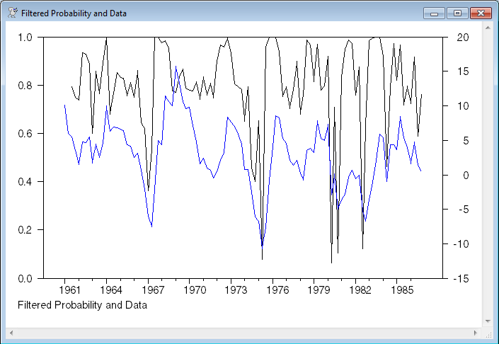
* Compute the probability of the regimes at each time period.
*
set pt_t = f=RegimeF(t),p*f(1)/(p*f(1)+(1-p)*f(2))
graph(footer="Filtered Probability and Data",overlay=line) 2
# pt_t
# x
*
* EM
*
frml emlogl = f=RegimeF(t),pt_t*log(p*f(1))+(1-pt_t)*log((1-p)*f(2))
*
function EStep
set pt_t = f=RegimeF(t),p*f(1)/(p*f(1)+(1-p)*f(2))
end
*
* Reset the guess values.
*
compute %parmspoke(regparms,guesses)
compute p=.3
*
* Do 50 EM iterations, then switch over to ML. (EM itself doesn't
* converge in even 500 iterations). Note that the EM log likelihood
* isn't comparable to the ML log likelihood.
*
maximize(estep=Estep(),method=bhhh,parmset=regparms+msparms,iters=50) emlogl rstart rend
maximize(method=bfgs,parmset=regparms+msparms,hessian=%xx) logl rstart rend
*
* Bayesian MCMC
* Note that this has a severe "labeling" problem---the model doesn't
* really want to separate the regimes in the way that we intend.
*
compute %parmspoke(regparms,guesses)
compute p=.3
*
compute r1=r2=5
compute pdf=1,pscale=0.0
compute nburn=1000,ndraws=1000
dec series[integer] s
dec vect[vect] bphi(2)
dec vect[symm] hphi(2)
compute bphi(1)=phi(1)
compute bphi(2)=phi(2)
compute hphi(1)=%diag(||0.0,0.0,0.0||)
compute hphi(2)=%diag(||0.0,0.0,0.0||)
*
* Smallest regime size
*
compute minsize=5
*
set pstar rstart rend = 0.0
infobox(action=define,progress,lower=-nburn,upper=ndraws) "Gibbs sampling"
do draw=-nburn,ndraws
   *
   * Draw regimes given regression parameters and p. If the size of either regime is too small, reject and redraw.
   *
:redrawregimes
   gset s rstart rend = f=RegimeF(t),%ranbranch(||p*f(1),(1-p)*f(2)||)
   sstats rstart rend (s==1)>>count1 (s==2)>>count2
   if count1<minsize.or.count2<minsize {
      disp "Draw" draw "Redrawing regimes with regime of size" $
         %min(count1,count2)
      goto redrawregimes
   }
   *
   * Draw p given s
   *
   sstats rstart rend s==1>>count1
   compute p=%ranbeta(count1+r1,%nobs-count1+r2)
   *
   * Draw phi's given s, sigsq
   *
   cmom(smpl=(s==1),equation=xeq) rstart rend
   compute phi(1)=%ranmvpostcmom(%cmom,1.0/sigsq,hphi(1),bphi(1))
   cmom(smpl=(s==2),equation=xeq) rstart rend
   compute phi(2)=%ranmvpostcmom(%cmom,1.0/sigsq,hphi(2),bphi(2))
   *
   * Relabel if necessary
   *
   if phi(1)(1)<phi(2)(1) {
      disp "Relabel"
      compute temp=phi(1)
      compute phi(1)=phi(2)
      compute phi(2)=phi(1)
      gset s = 3-s
   }
   *
   * Draw sigsq given phi's and s
   *
   sstats rstart rend %eqnrvalue(xeq,t,phi(s))^2>>%rss
   compute sigsq=(pscale*pdf+%rss)/%ranchisqr(%nobs+pdf)
   infobox(current=draw)
   if draw>0
      set pstar rstart rend = pstar+(s==1)
end do draw
infobox(action=remove)
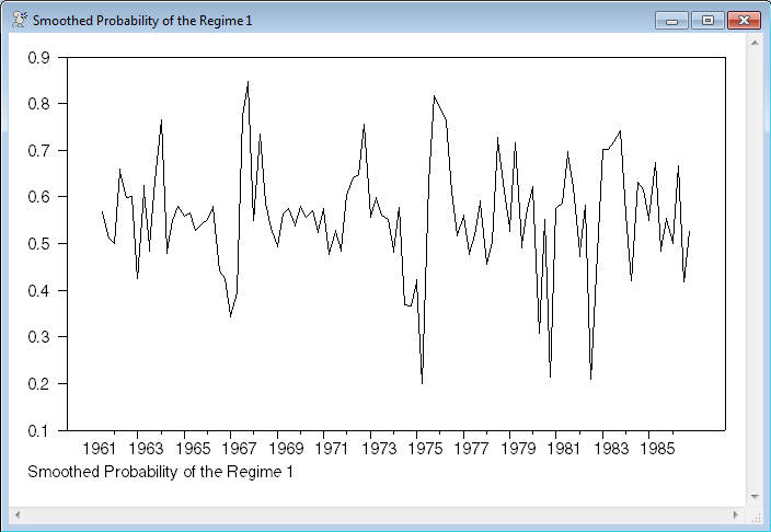
set pstar rstart rend = pstar/ndraws
graph(footer="Smoothed Probability of the Regime 1")
# pstar

Output

Linear Regression - Estimation by Least Squares

Dependent Variable X

Quarterly Data From 1961:03 To 1986:04

Usable Observations 102

Degrees of Freedom 99

Centered R^2 0.6453948

R-Bar^2 0.6382310

Uncentered R^2 0.7405378

Mean of Dependent Variable 2.8792264706

Std Error of Dependent Variable 4.7781935368

Standard Error of Estimate 2.8739512210

Sum of Squared Residuals 817.69996644

Regression F(2,99) 90.0919

Significance Level of F 0.0000000

Log Likelihood -250.8894

Durbin-Watson Statistic 2.0443

Variable Coeff Std Error T-Stat Signif

************************************************************************************

1. Constant 0.597900405 0.340330078 1.75683 0.08203946

2. X{1} 0.883534978 0.099660714 8.86543 0.00000000

3. X{2} -0.102956987 0.098634700 -1.04382 0.29911029

MAXIMIZE - Estimation by BFGS

Convergence in 26 Iterations. Final criterion was 0.0000068 <= 0.0000100

Quarterly Data From 1961:03 To 1986:04

Usable Observations 102

Function Value -249.0669

Variable Coeff Std Error T-Stat Signif

************************************************************************************

1. PHI(1)(1) 1.330046906 0.675662810 1.96851 0.04900974

2. PHI(1)(2) 0.883937946 0.115827682 7.63149 0.00000000

3. PHI(1)(3) -0.163415020 0.104765464 -1.55982 0.11880298

4. PHI(2)(1) -2.846215075 1.874403708 -1.51846 0.12889740

5. PHI(2)(2) 0.563569215 0.597564424 0.94311 0.34562444

6. PHI(2)(3) 0.545576875 0.558193588 0.97740 0.32837253

7. SIGSQ 6.129982723 1.105078681 5.54710 0.00000003

8. P 0.791252950 0.228636730 3.46074 0.00053869

MAXIMIZE - Estimation by BHHH

NO CONVERGENCE IN 50 ITERATIONS

LAST CRITERION WAS 0.0125456

Quarterly Data From 1961:03 To 1986:04

Usable Observations 102

Function Value -314.8333

Variable Coeff Std Error T-Stat Signif

************************************************************************************

1. PHI(1)(1) 1.315154823 4.505065125 0.29193 0.77034165

2. PHI(1)(2) 0.939725914 0.368147741 2.55258 0.01069289

3. PHI(1)(3) -0.157931310 0.448460738 -0.35216 0.72471597

4. PHI(2)(1) -1.001211875 4.469197093 -0.22402 0.82273785

5. PHI(2)(2) 0.754966034 0.646670945 1.16747 0.24302242

6. PHI(2)(3) 0.158487702 1.085903259 0.14595 0.88396077

7. SIGSQ 8.585740318 5.448614057 1.57577 0.11507976

8. P 0.590332476 1.546262915 0.38178 0.70262445

MAXIMIZE - Estimation by BFGS

Convergence in 16 Iterations. Final criterion was 0.0000036 <= 0.0000100

Quarterly Data From 1961:03 To 1986:04

Usable Observations 102

Function Value -249.0669

Variable Coeff Std Error T-Stat Signif

************************************************************************************

1. PHI(1)(1) 1.330046492 0.683584819 1.94569 0.05169158

2. PHI(1)(2) 0.883938420 0.129079713 6.84800 0.00000000

3. PHI(1)(3) -0.163415342 0.114518886 -1.42697 0.15358772

4. PHI(2)(1) -2.846205749 1.873783196 -1.51896 0.12877202

5. PHI(2)(2) 0.563575218 0.610654231 0.92290 0.35605725

6. PHI(2)(3) 0.545573715 0.567459377 0.96143 0.33633490

7. SIGSQ 6.129996881 1.168978683 5.24389 0.00000016

8. P 0.791253272 0.234690466 3.37148 0.00074767

Graphs