MONTEVAR.RPF

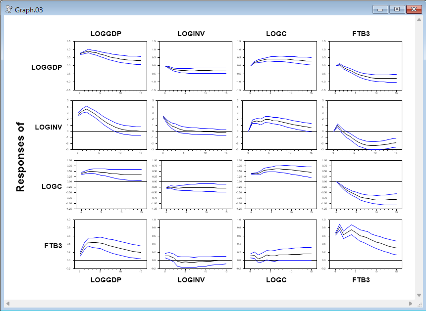
MONTEVAR.RPF is an example of Monte Carlo Integration of Impulse Responses. The technical details are covered in the linked section. Note that this is for illustration of the technique. In practice, you would use the @MONTEVAR procedure to do the draws.

The example is a four variable, four lag VAR with quarterly data. The variables are 100 x logs of real GDP, real investment and real consumption and the 3-month Treasury Bill rate. The impulse responses are computed for 16 steps (4 years), with 10000 draws of the Monte Carlo procedure. Those are all controlled by the first few lines, which initialize the variables used in the program.

Only the part above the line of ***'s are specific to the analysis of these data. Everything after that is standard.

Full Program

compute lags=4 ;*Number of lags

compute nstep=16 ;*Number of response steps

compute ndraws=10000 ;*Number of keeper draws

*
open data haversample.rat
cal(q) 1959
data(format=rats) 1959:1 2006:4 ftb3 gdph ih cbhm
*
set loggdp = 100.0*log(gdph)
set loginv = 100.0*log(ih)
set logc   = 100.0*log(cbhm)
*
system(model=varmodel)
variables loggdp loginv logc ftb3
lags 1 to lags
det constant
end(system)
******************************************************************
estimate
*
compute nvar   =%nvar
compute fxx    =%decomp(%xx)
compute fwish =%decomp(inv(%nobs*%sigma))
compute wishdof=%nobs-%nreg
compute betaols=%modelgetcoeffs(varmodel)
*
*
declare vect[rect] %%responses(ndraws)
*
infobox(action=define,progress,lower=1,upper=ndraws) $
   "Monte Carlo Integration"
do draw=1,ndraws
   *
   * On the odd values for <<draw>>, a draw is made from the inverse Wishart
   * distribution for the covariance matrix. This assumes use of the
   * Jeffrey's prior |S|^-(n+1)/2 where n is the number of equations in
   * the VAR. The posterior for S with that prior is inverse Wishart with
   * T-p d.f. (p = number of explanatory variables per equation) and
   * covariance matrix inv(T(S-hat)).
   *
   * Given the draw for S, a draw is made for the coefficients by adding
   * the mean from the least squares estimate to a draw from a
   * multivariate Normal with (factor of) covariance matrix as the
   * Kroneker product of the factor of the draw for S and a factor of
   * the X'X^-1 from OLS.
   *
   * On even draws, the S is kept at the previous value, and the
   * coefficient draw is reflected through the mean.
   *
   if %clock(draw,2)==1 {
      compute sigmad =%ranwisharti(fwish,wishdof)
      compute fsigma =%decomp(sigmad)
      compute betau   =%ranmvkron(fsigma,fxx)
      compute betadraw=betaols+betau
   }
   else
      compute betadraw=betaols-betau
   *
   * Push the draw for the coefficient back into the model.
   *
   compute %modelsetcoeffs(varmodel,betadraw)
   *
   * Compute the IRF's and "flatten" them into element DRAW of the
   * %%RESPONSES array.
   *
   impulse(noprint,model=varmodel,factor=fsigma,$
     results=impulses,steps=nstep,flatten=%%responses(draw))
   infobox(current=draw)
end do draw
infobox(action=remove)
*
@mcgraphirf(model=varmodel)

Graph