ONEBREAK.RPF

ONEBREAK.RPF analyzes a linear regression with single break in time sequence. It is based on an example from Stock & Watson (2011), Chapter 15. The model being estimated is a long distributed lag of the percentage change in the relative price of Orange Juice (OJ price divided by the overall PPI) on the “Freezing Degree Days”, which is a measure of low temperatures in the growing region.

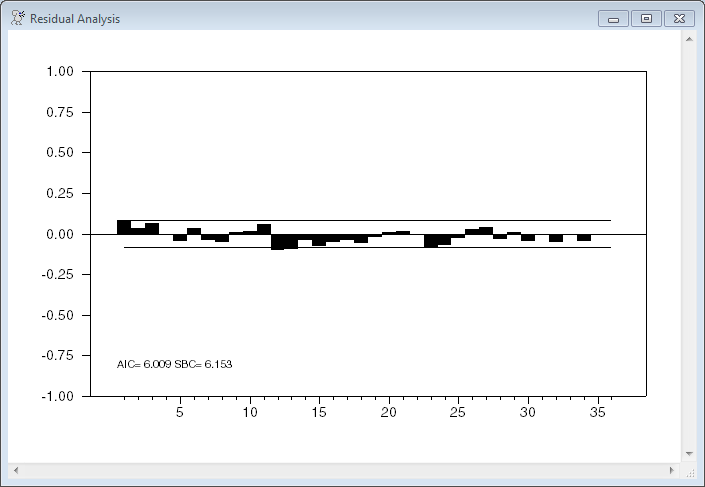
The model is estimated by least squares. If we assumed homoscedastic errors, we could use the @APBreakTest procedure (which the example uses as well). However, the authors want to correct the covariance matrix for possible serial correlation using a Newey-West window. There’s no short-cut way to do the sequential tests under those conditions—you have to estimate the model with both the original variables and the dummied-out versions.

This uses a one-break structure, searching for the maximal F-statistic. It also graphs the series of break statistics, as does the @APBreakTest procedure. As you can see, there is quite a bit of difference between the patterns with and without correction for serial correlation.

This part does the @APBreakTest, which looks for a single break (in the time sequence) for a standard linear regression:

@apbreaktest(graph) drpoj 1950:1 2000:12

# constant fdd{0 to 18}

This estimates the target regression over the full data set with the desired Newey-West standard errors and checks for serial correlation in the residuals:

linreg(lags=7,lwindow=newey,define=baseeqn) drpoj 1950:1 2000:12

# constant fdd{0 to 18}

@regcorrs(number=36)

This is the “one-break” setup code described in the User's Guide. The upper and lower bounds are pulled out from the full sample regression using %REGSTART() and %REGEND().

compute lower=%regstart(),upper=%regend()

compute pi=.15

compute nobs =upper-lower+1

compute bstart=lower+fix(pi*nobs)

compute bend =upper-fix(pi*nobs)

FSTAT will be used for a graph of the test statistics.

set fstat lower upper = %na

DUMMIES will have the dummied-out copies of the original regressors. For each value of TIME, this will reset the dummies for the subsample greater than TIME. This uses %EQNXVECTOR to extract the full $x_t$ vector, then pulls out element I from it. After the dummies are generated, this runs the regression (with the original regression plus the dummies) and gets the F-statistic on the dummies. Under these circumstances (with a HAC covariance matrix), EXCLUDE will give a chi-squared test with K degrees of freedom. According to the recommendation in the book, this is transformed into an approximate F statistic.

compute k=%nreg

dec vect[series] dummies(k)

compute maxf=%na

do time=bstart,bend

do i=1,k

set dummies(i) = %eqnxvector(baseeqn,t)(i)*(t>time)

end do i

linreg(noprint,lags=7,lwindow=newey) drpoj lower upper

# constant fdd{0 to 18} dummies

exclude(noprint)

# dummies

compute fac = float(%ndf)/float(%nobs)

compute fstat(time) = %cdstat*fac/k

if fstat(time)>maxf

compute maxf=fstat(time),bestbreak=time

end do

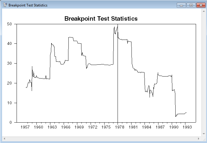
This graphs the F statistics, with a GRID value at the time of the largest break.

graph(grid=(t==bestbreak),$

header="Robust F-Statistics for Breakpoints")

# fstat

Full Program

*
* The model being estimated is a long distributed lag of the percentage
* change in the relative price of Orange Juice (OJ price divided by the
* overall PPI) on the "Freezing Degree Days", a measure of low
* temperatures in the growing region.
*
cal(m) 1947:1
*
open data ch15_oj.rat
data(format=rats) 1947:1 2001:12 ppioj pwfsa fdd
*
set poj   = ppioj/pwfsa
set rpoj = log(poj)
set drpoj = rpoj-rpoj{1}
set drpoj = 100*drpoj
*
* APBreakTest will do a test for breaks in the specification, but can't
* do the test using the desired Newey-West correction.
*
@apbreaktest(graph) drpoj 1950:1 2000:12
# constant fdd{0 to 18}
*
* This is the regression of interest. To allow for the serial
* correlation in the residuals, this employs a Newey-West correction
* with 7 lags.
*
linreg(lags=7,lwindow=newey,define=baseeqn) drpoj 1950:1 2000:12
# constant fdd{0 to 18}
@regcorrs(number=36)
*
* This does the break test using F-statistics applied to the regressions
* with Newey-West corrections. Because the covariance matrix calculation
* needs residuals from more than one observation, there's no real
* alternative to brute force calculation of the regression with dummies.
*
compute lower=%regstart(),upper=%regend()
compute pi=.15
*
compute nobs =upper-lower+1
compute bstart=lower+fix(pi*nobs)
compute bend =upper-fix(pi*nobs)
*
* <<fstat>> will be used for a graph of the test statistics.
*
set fstat lower upper = %na
*
* <<dummies>> will have the dummied-out copies of the original
* regressors.
*
compute k=%nreg
dec vect[series] dummies(k)
*
compute maxf=%na
*
do time=bstart,bend
   *
   * Set up the dummies
   *
   do i=1,k
      set dummies(i) = %eqnxvector(baseeqn,t)(i)*(t>time)
   end do i
   *
   * Do the regression and get the F-statistic on the dummies.
   *
   linreg(noprint,lags=7,lwindow=newey) drpoj lower upper
   # constant fdd{0 to 18} dummies
   exclude(noprint)
   # dummies
   *
   * EXCLUDE will give a chi-squared test with <<k>> degrees of freedom.
   * This is transformed into a approximate F statistic.
   *
   compute fac = float(%ndf)/float(%nobs)
   compute fstat(time) = %cdstat*fac/k
   if fstat(time)>maxf
      compute maxf=fstat(time),bestbreak=time
end do
*
graph(grid=(t==bestbreak),header="Robust F-Statistics for Breakpoints")
# fstat

Output

Linear Regression - Estimation by Least Squares

Dependent Variable DRPOJ

Monthly Data From 1950:01 To 2000:12

Usable Observations 612

Degrees of Freedom 592

Centered R^2 0.1285029

R-Bar^2 0.1005325

Uncentered R^2 0.1289590

Mean of Dependent Variable -0.115821495

Std Error of Dependent Variable 5.065299457

Standard Error of Estimate 4.803943096

Sum of Squared Residuals 13662.098605

Regression F(19,592) 4.5943

Significance Level of F 0.0000000

Log Likelihood -1818.7188

Durbin-Watson Statistic 1.8212

Variable Coeff Std Error T-Stat Signif

************************************************************************************

1. Constant -0.340237075 0.253258141 -1.34344 0.17964433

2. FDD 0.503798561 0.060511024 8.32573 0.00000000

3. FDD{1} 0.169918304 0.060507198 2.80823 0.00514572

4. FDD{2} 0.067013958 0.060500556 1.10766 0.26845914

5. FDD{3} 0.071086493 0.060501593 1.17495 0.24048611

6. FDD{4} 0.024776594 0.060493134 0.40958 0.68226445

7. FDD{5} 0.031934791 0.060476057 0.52806 0.59765782

8. FDD{6} 0.032560686 0.059759856 0.54486 0.58605579

9. FDD{7} 0.014913302 0.059104122 0.25232 0.80087935

10. FDD{8} -0.042197057 0.058856826 -0.71694 0.47369132

11. FDD{9} -0.010299171 0.058865490 -0.17496 0.86117003

12. FDD{10} -0.116300723 0.058856826 -1.97599 0.04861934

13. FDD{11} -0.066282894 0.059104122 -1.12146 0.26254689

14. FDD{12} -0.142267779 0.059759856 -2.38066 0.01759714

15. FDD{13} -0.081575439 0.060476057 -1.34889 0.17788861

16. FDD{14} -0.056372627 0.060493134 -0.93188 0.35177598

17. FDD{15} -0.031875052 0.060501593 -0.52685 0.59849754

18. FDD{16} -0.006777476 0.060500556 -0.11202 0.91084285

19. FDD{17} 0.001394167 0.060507198 0.02304 0.98162506

20. FDD{18} 0.001823530 0.060511024 0.03014 0.97596914

Andrews-Quandt Andrews-Ploberger

Test P-Val Date Test P-Val

Constant 1.096753 0.988 1964:04 0.059178 1.000

FDD 14.468254 0.003 1977:02 5.246633 0.000

FDD{1} 9.415627 0.035 1980:04 2.803746 0.020

FDD{2} 2.009584 0.783 1964:04 0.312641 0.627

FDD{3} 6.407517 0.134 1963:04 1.697738 0.077

FDD{4} 0.766939 1.000 1957:08 0.045725 1.000

FDD{5} 3.102897 0.533 1958:06 0.575573 0.386

FDD{6} 2.221923 0.731 1977:09 0.343815 0.590

FDD{7} 0.998070 0.999 1957:08 0.073457 1.000

FDD{8} 2.283291 0.716 1984:09 0.408079 0.521

FDD{9} 1.362694 0.939 1978:12 0.207215 0.783

FDD{10} 11.893434 0.011 1990:01 3.776896 0.005

FDD{11} 2.263972 0.721 1957:08 0.153507 0.888

FDD{12} 15.360685 0.002 1970:01 5.387221 0.000

FDD{13} 2.884863 0.578 1957:08 0.245376 0.720

FDD{14} 1.170846 0.976 1957:08 0.324704 0.612

FDD{15} 0.821271 1.000 1991:04 0.097078 1.000

FDD{16} 3.880227 0.393 1959:06 0.644851 0.343

FDD{17} 0.731948 1.000 1957:08 0.083878 1.000

FDD{18} 0.889715 1.000 1957:08 0.100320 1.000

All Coeffs 48.699960 0.010 1978:01 20.405606 0.009

Resid Var 5.421638 0.207 1967:02 1.908781 0.059

Linear Regression - Estimation by Least Squares

HAC Standard Errors with Newey-West/Bartlett Window and 7 Lags

Dependent Variable DRPOJ

Monthly Data From 1950:01 To 2000:12

Usable Observations 612

Degrees of Freedom 592

Centered R^2 0.1285029

R-Bar^2 0.1005325

Uncentered R^2 0.1289590

Mean of Dependent Variable -0.115821495

Std Error of Dependent Variable 5.065299457

Standard Error of Estimate 4.803943096

Sum of Squared Residuals 13662.098605

Log Likelihood -1818.7188

Durbin-Watson Statistic 1.8212

Variable Coeff Std Error T-Stat Signif

************************************************************************************

1. Constant -0.340237075 0.269150136 -1.26412 0.20618829

2. FDD 0.503798561 0.137263828 3.67029 0.00024227

3. FDD{1} 0.169918304 0.087478100 1.94241 0.05208753

4. FDD{2} 0.067013958 0.059692495 1.12265 0.26158490

5. FDD{3} 0.071086493 0.044153975 1.60997 0.10740481

6. FDD{4} 0.024776594 0.031134455 0.79579 0.42615212

7. FDD{5} 0.031934791 0.030256200 1.05548 0.29120620

8. FDD{6} 0.032560686 0.046817429 0.69548 0.48675319

9. FDD{7} 0.014913302 0.015483153 0.96320 0.33544948

10. FDD{8} -0.042197057 0.034310093 -1.22987 0.21874467

11. FDD{9} -0.010299171 0.050604141 -0.20352 0.83872528

12. FDD{10} -0.116300723 0.069491500 -1.67360 0.09420995

13. FDD{11} -0.066282894 0.052140883 -1.27123 0.20364793

14. FDD{12} -0.142267779 0.076148278 -1.86830 0.06172035

15. FDD{13} -0.081575439 0.042284123 -1.92922 0.05370337

16. FDD{14} -0.056372627 0.034718305 -1.62371 0.10443668

17. FDD{15} -0.031875052 0.027556601 -1.15671 0.24739002

18. FDD{16} -0.006777476 0.054783627 -0.12371 0.90154210

19. FDD{17} 0.001394167 0.018141206 0.07685 0.93874221

20. FDD{18} 0.001823530 0.016693770 0.10923 0.91301676

Graphs