QPLOT Procedure

@QPlot creates a Q plot for a series against a hypothesized distribution.

@QPlot( options ) series start end

Parameters

series	series to graph
start, end	range of series to graph. By default, the defined range of series.

Options

DISTRIB=[NORMAL]/EXPONENTIAL

Determines the comparison distribution

TITLE=" descriptive title for graph " [none]

MEAN=mean for comparison distribution [sample mean]

This applies to either comparison distribution.

STDDEV=standard deviation for comparison distribution [sample standard error]

This applies to either the Normal.

BOUND=lower bound for exponential distribution [0]

Example

* Brockwell & Davis, Introduction to Time Series and Forecasting, 2nd ed.

* Examples 5.2.5 and 5.3.3 from pp 164-167

open data lake.dat

cal 1875

data(format=free,org=columns) 1875:1 1972:1 lake

boxjenk(ar=1,ma=1,demean,maxl) lake

* Graph the residuals

graph(footer="Figure 5.5 Rescaled Residuals from ARMA(1,1) model")

# %resids

* REGCORRS is a procedure for doing a correlation analysis on residuals.

@regcorrs(number=40)

@bdindtests(number=22) %resids

* You can get the Jarque-Bera normality test as part of the output from a

* STATISTICS instruction.

stats %resids

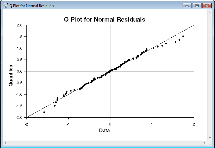
@qplot(title="Q Plot for Normal Residuals") %resids

Sample Output