UNITROOTBREAK.RPF

UNITROOTBREAK.RPF is an example of unit root tests with breaks. This includes a standard Dickey-Fuller test (@DFUNIT) and three different testings procedures which allow for breaks: @LSUNIT (Lee-Strazicich), @LPUNIT (Lumsdaine-Papell, though this is actually the same as Zivot-Andrews with these options) and @PERRONBREAKS. The Lee-Strazicich and Lumsdaine-Papell papers are about double breaks, but here we're just allowing for one. Note that these handle the break in different ways, so they will tend to pick different locations for it. And a reminder that these are tests for unit roots (allowing for breaks), not a test for breaks. The Dickey-Fuller test fails to reject the unit root. If it rejected it, the remainder of the analysis would be fairly pointless.

All three procedures with breaks allow for a simultaneous break in the level and the trend rate. (This is controlled by a differently named option on each). The @LSUNIT and @LPUNIT choose the augmenting lag length by GTOS pruning, while the @PERRONBREAKS uses AIC⎯the additive outlier model adds two parameters per lag, so it's better to use an information criterion for lag length choice.

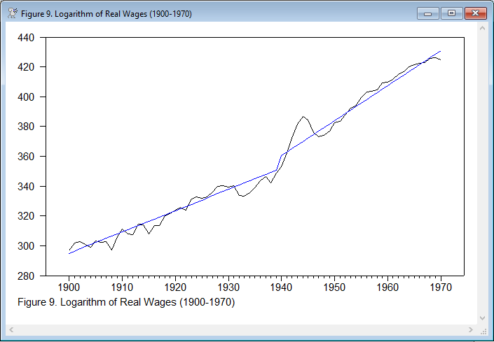
Finally, it uses @GLSDETREND to do a local-to-unity detrending with a break in level and trend rate at the consensus break date of 1939:1. That procedure produces the detrended data, so that's subtracted off from the actual to give the broken trend, which is graph with the actual data.

Full Program

open data nelsonplosser.rat
calendar(a) 1871
data(format=rats) 1871:1 1970:1 realwages stockprice
*
set logwage = 100.0*log(realwages)
*
@dfunit(det=trend,maxlag=8,method=gtos) logwage
@lsunit(model=break,lags=8,method=gtos,breaks=1) logwage
@lpunit(break=both,maxlags=8,method=gtos,nbreaks=1) logwage
@perronbreaks(ao=breaks,breaks=1,lags=8,method=aic) logwage
*
* Figures with detrended data
*
@glsdetrend(break=both,tb=1939:1) logwage / wagedetrend
set wagetrend = logwage-wagedetrend
graph(footer="Figure 9. Logarithm of Real Wages (1900-1970)") 2
# logwage
# wagetrend

Output

Dickey-Fuller Unit Root Test, Series LOGWAGE

Regression Run From 1902:01 to 1970:01

Observations 70

With intercept and trend

With 1 lags chosen from 8 by GTOS/t-tests(0.100)

Sig Level Crit Value

1%(**) -4.09281

5%(*) -3.47394

10% -3.16399

T-Statistic -3.04861

Lee-Strazicich Unit Root Test, Series LOGWAGE

Regression Run From 1909:01 to 1970:01

Observations 62

Trend Break Model with 1 breaks

With 3 lags chosen from 8

Variable Coefficient T-Stat

S{1} -0.6073 -5.3705

Constant 0.7557 1.3032

D(1939:01) -5.2148 -1.5137

DT(1939:01) 6.7523 4.9291

Lumsdaine-Papell Unit Root Test, Series LOGWAGE

Regression Run From 1903:01 to 1970:01

Observations 69

Breaks in Intercept and Trend

Breaks at 1940:01

With 1 lags chosen from 8

Selected by GTOS/t-tests(0.10)

Sig Level Crit Value

1%(**) -5.5700

5%(*) -5.0800

10% -4.8200

Variable Coefficient T-Stat

Y{1} -0.4550 -5.1283

D(1940:01) 7.5369 3.9724

DT(1940:01) 0.2995 2.5781

Constant 114.6974 5.0768

Trend 0.6434 5.0686

Unit Root Test, Series LOGWAGE

Regression Run From 1909:01 to 1970:01

Observations 70

AO Model: Full Trend Break with 1 breaks

With 2 lags chosen from 8

Selection by BIC

Variable Coefficient T-Stat

Y{1} -0.482577 -4.258754

Break point(s)

1939:01

Graph