FILTER( options )   series start end newseries newstart

#  list of lags in filter

#  list of corresponding filter coefficients

 

FILTER passes a series through a linear filter. It includes a wide variety of standard filters, or you can provide the form of the filter yourself, either with a pair of supplementary cards or with an EQUATION. FILTER also includes an option for removing the trend or seasonal from a series by linear regression.

 

DIFFERENCE does a specific set of differencing and fractional differencing filters. In addition the techniques provided by FILTER and DIFFERENCE, there are many RATS procedures available that implement other filtering techniques.

Wizard

You can use the Data/Graphics—Filter/Smooth Wizard to do various filtering operations. Choose which technique to apply using the "Filter Type" drop down.

Parameters

Options

TYPE=[GENERAL]/FLAT/HENDERSON/SPENCER/HP/HPDETREND/LAGGING/CENTERED

WIDTH=base window width of filter [1 (15 when using TYPE=HENDERSON)]

BY=repetitions of simpler filter (used with TYPE=FLAT)

TUNING=tuning value for TYPE=HP or TYPE=HPDETREND [depends on CALENDAR]

TYPE indicates the type of filter to be used. See "Technical Information".

 

TYPE=GENERAL (the default) allows any pattern—if used, it requires use of either the supplementary cards or the EQUATION option to indicate the form of the filter. With TYPE=GENERAL, the zero lag is assumed to have a coefficient of 1.0 unless included explicitly.

TYPE=FLAT is a centered flat moving average, with width given by WIDTH. It can also be used for an NxM convolution of flat filters, by combining the WIDTH and BY options.

TYPE=HENDERSON gives a centered Henderson filter with width given by the WIDTH option. This filter is used extensively by the X11 seasonal adjustment procedure.

TYPE=HP implements the Hodrick-Prescott filter. You can use the TUNING option to supply a value for the tuning parameter for the HP filter. The default values for this depend on the frequency of the current CALENDAR setting (100 for annual data, 1,600 for quarterly, and 14,400 for monthly).

 

TYPE=HPDETREND produces the residuals from the Hodrick-Prescott filter (generally interpreted as the "cycle"). The TUNING option applies as it does for TYPE=HP.

TYPE=SPENCER does the Spencer moving average filter. WIDTH must be 15 or 21 (the default is 15)

TYPE=LAGGING gives a filter on a list of lags. If you use the WEIGHTS option, it will use those values. Otherwise it will put equal weights on the lags 0 through \(L-1\), given WIDTH=L.
 

TYPE=CENTERED is the same as TYPE=FLAT, except that you can supply filter weights with the WEIGHTS option. Note that for TYPE=CENTERED, you only need to supply the weights for half the window, starting with 0 lag and working out—the same lag weights will automatically be used for the leads.
 

WEIGHTS=VECTOR of filter weights

UNITSUM/[NOUNITSUM] (Used with WEIGHTS)

WEIGHTS provides the filter weights used with the TYPE=LAGGING or TYPE=CENTERED options. Use UNITSUM if you want FILTER to normalize the WEIGHTS to sum to 1—this allows you to just supply a shape using WEIGHTS and let FILTER figure out the normalization. For example: TYPE=CENTERED, WEIGHTS=||5.0,3.0,2.0||,UNITSUM gives filter coefficients: 2/15, 3/15, 5/15, 3/15, 2/15.
 

REMOVE=MEAN/TREND/SEASONAL/BOTH [unused]

On the first four choices, removes from series by linear regression the mean, mean and trend, seasonal (using dummies) and mean, or trend and seasonals, respectively. This is not technically a linear filter, but serves a similar purpose to many of the other filters.

 

EQUATION=equation which forms filter [unused]

The form of a GENERAL filter comes from the equation—see “Using the EQUATION Option”. Omit the supplementary cards when you use it.

 

TRUNCATE/[NOTRUNCATE]

EXTEND=ZEROS/REPEAT/RESCALE/MSEREWEIGHT

If you set start and end manually, you normally need to allow for lags and leads. For example, if your filter includes lags, you could not start at entry one, since the lag terms would refer to non-existent entries. TRUNCATE and EXTEND offer two alternative ways to handle out-of-sample values.
 

With TRUNCATE, you can specify any start and end values. RATS will assume that all unavailable entries outside the data range are equal to 0 for the purposes of computing the filtered series (Missing values in the middle of the data are still treated as missing).

 

EXTEND=ZEROS is identical to TRUNCATE. EXTEND=REPEAT repeats the nearest end-point value. EXTEND=RESCALE uses available data, but reweights the filter coefficients near the endpoints to maintain the sum of weights. For example, a centered filter with weights (1/4, 1/2, 1/4) will be reweighted as (1/3, 2/3) at the left end point. EXTEND=MSEREWEIGHT implements the minimum mean square revision technique—the same method used for the Henderson Moving Average terms in the Census X13 Seasonal Adjustment process (see Findley, et al 1998).

Supplementary Cards

You need two supplementary cards unless you use one of the pre-defined filter types, or the EQUATION option. Note that TYPE=CENTERED or LAGGING with input WEIGHTS will usually be simpler than using these.

1.The first lists the lags in the filter. Represent leads as negative numbers. In filters which involve lags only, lag 0 gets a coefficient of 1.0 unless you set it explicitly.

2.The second lists the filter coefficients. They correspond, in order, to the lags on the first card.

Missing Values

If any of the values required to compute an entry are missing, FILTER sets the entry in the output series to missing. Exception: data that are unavailable at the beginning or end of the filter are treated differently when using TRUNCATE or EXTEND options.

Technical Information

For TYPE=FLAT, if the window size is odd (WIDTH=2N+1), the filtered series is
 

\({\tilde x_t} = \frac{1}{{\left( {2N + 1} \right)}}\left( {{x_{t - N}} + {x_{t - N + 1}} +  \ldots  + {x_{t + N - 1}} + {x_{t + N}}} \right)\)

 

If it’s even (WIDTH=2N), the output is
 

\({\tilde x_t} = \frac{1}{{\left( {2N} \right)}}\left( {0.5{x_{t - N}} + {x_{t - N + 1}} +  \ldots  + {x_{t + N - 1}} + 0.5{x_{t + N}}} \right)\)

 

This is generally used with seasonal data where the WIDTH is the length of the seasonal, and is also known as a 2xN filter.

 

If TYPE=FLAT and you use both the WIDTH and BY options, the result is the same effect as a flat filter of width given by the WIDTH applied to the output of a flat filter of width given by the BY option. This concentrates the filter a bit more towards the center than a flat filter of the same overall length.

 

A Henderson filter (TYPE=HENDERSON) is a centered filter whose lag coefficients are selected to minimize the sum of squared third differences of the lag coefficients for the class of symmetric lag polynomials which pass third order polynomials through without change. It’s used within the X11 adjustment procedure to estimate local trends. The width should be odd, and is rounded up if the WIDTH option is even.

 

A Spencer filter (TYPE=SPENCER) is similar to the Henderson filter, but allows only the two widths (15 and 21).

 

The Hodrick-Prescott Filter (Hodrick and Prescott, 1997) computes the estimated growth component \(g\) of a series \(x\) that minimizes the sum over \(t\) of:

 

\({\left( {{x_t} - {g_t}} \right)^2} + \lambda {\left( {{g_t} - 2{g_{t - 1}} + {g_{t - 2}}} \right)^2}\)       

 

The value of \(\lambda\) is set by the TUNING option. This is solved internally by Kalman smoothing. The two choices that use this are TYPE=HP (which returns the growth component itself, and TYPE=HPDETREND which returns the difference between the actual data and the computed growth component. See the HPFILTER.RPF example for additional technical details.

Examples

This computes the 3 and 5 period moving averages of inflation (using current and two lags and current and four lags, respectively)

 

filter(type=lagging,span=3) pceinflation / pi3

filter(type=lagging,span=5) pceinflation / pi5

data 1955:1 2010:6 ip

filter(type=flat,width=12) ip 1955:7 2009:12 trdcycle               

 

This sets \(TRDCYCL{E_t} = \left( {.5 \times I{P_{t - 6}} + I{P_{t - 5}} +  \ldots I{P_{t + 5}} + .5 \times I{P_{t + 6}}} \right)/12\) . Note that the range is set to run from (1955:1)+6 to (2010:6)–6. This use of an even window size means that each calendar month will get the same weight in the average, and thus a seasonal will tend to be flattened.

 

filter(type=lagging,weights=||4,3,2,1||,unitsum) data / wma

 

computes \(WM{A_t} = .4 \times DATA_t + .3 \times DATA_{t - 1}} + .2 \times DATA_{t - 2}} + .1 \times DATA_{t - 3}}\), normalizing the 4,3,2,1 weight pattern to sum to 1.

 

 

filter(type=henderson,width=23,extend=mse) data / tc

 

does a 23-term Henderson with minimum MSE revision handling of the end points.

 

filter(remove=seasonal) van / deseas

filter(type=centered,width=5) deseas / trend

 

removes the seasonal from VAN by regression on seasonal dummies, then smooths with a five term centered moving average to get a simple estimate of the trend-cycle.

 

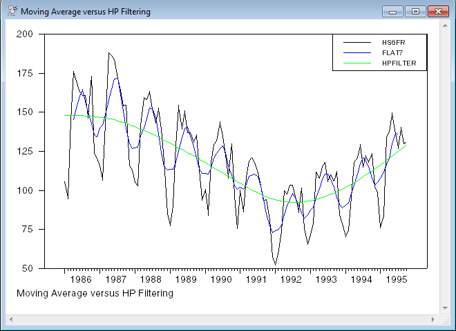
This does a centered 7 term moving average and an H-P filtered version of the series HS6FR. Note that the H-P filter returns the trend, not the deviation. If you want the H-P "cycle" subtract the trend from the original data.

 

The 7 term moving average without one of the EXTEND choices will lose 3 data points at each end of the data. You can see where the blue line in the graph cuts out a few data points earlier than the others.

 

open data ex152.xls

calendar(m) 1986:1

data(format=xls,org=columns) 1986:1 1995:10 hs6fr

*

* Computing filtered series using a 7-period moving average

* and the Hodrick-Prescott filter:

*

filter(type=centered,width=7) hs6fr / flat7

filter(type=hp) hs6fr / hpfilter

*

* Generate a graph comparing the original series and the

* two filtered series:

*

GRAPH(STYLE=LINE,FOOTER="Moving Average versus HP Filtering",KEY=UPRIGHT) 3

# HS6FR

# FLAT7

# HPFILTER

 

Sample Output

 

Using the EQUATION Option

The equation must have one of the following forms:

 

1.  \({y_t} = A\left( L \right)\,{y_t}\) (univariate autoregression)

 

2.  \({y_t} = B\left( L \right)\,{x_t}\) (univariate distributed lag)

 

The only other variable allowed in the equation is the CONSTANT. FILTER uses \(1-A\left( L \right)\) for type 1 and \(B\left( L \right)\) for type 2, for instance,

 

 

The variables in the equation do not have to be related to the series you are filtering. For instance, the equation in the next example is an autoregression on residuals, after which FILTER is applied to the dependent variable and regressors.

Example with EQUATION

This filters the series loggpop and logpg with a linear filter derived from a second order AR:

 

linreg(define=ar2) resids

# resids{1 2}

filter(equation=ar2) loggpop / fgpop

filter(equation=ar2) logpg   / fpg

Using Vectors

For long and complex filters, it is probably simplest to put the filter coefficients into a vector. The supplementary cards on FILTER will accept a vector of integers for the list of lags and vector of real numbers. For instance, the following generates a fifty lag expansion of a fractional difference filter. (Note that DIFFERENCE has an option for a specific form of fractional differencing).

 

dec vect[int] lags(50)

dec vect coeffs(50)

ewise lags(i)=i

ewise coeffs(i)=%binomial(.7,i)*(-1)^i

filter(truncate) series / fracdiffs

# lags

# coeffs

 

Copyright © 2025 Thomas A. Doan