IMPULSES.RPF

IMPULSES.RPF computes and graphs impulse response functions for a six variable VAR (to Cholesky shocks) in several different formats. Two are done using the procedure @VARIRF, which does one page per shock and one page per variable (again with six panes). Then, direct programming is used to do single graphs with responses of all six variables to each shock, and single graphs with responses for each variable to all shocks. It also uses @MONTEVAR to do a basic set of confidence bands. If you’re interested in a more involved setup for standard error bands or some other type of confidence limit on the estimates, see Monte Carlo Integration: VAR's.

Five of the series are in logs, while interest rates are kept in levels. (This is a model for Canadian data, with "open economy" features, as it includes also US real GDP and the Canadian $/US $ exchange rate.) The logged series are all scaled by 100, which gives the responses a more natural scale—a response of 3 would be interpreted as 3% increase over the baseline due to the shock and -2 would be a 2% decrease. For the interest rate, which is in percent per annum, a response of 1 means a 1 percentage point increase (for instance, 5% to 6%).

open data oecdsample.rat

calendar(q) 1981

data(format=rats) 1981:1 2006:4 can3mthpcp canexpgdpchs canexpgdpds $

canm1s canusxsr usaexpgdpch

set logcangdp = 100.0*log(canexpgdpchs)

set logcandefl = 100.0*log(canexpgdpds)

set logcanm1 = 100.0*log(canm1s)

set logusagdp = 100.0*log(usaexpgdpch)

set logexrate = 100.0*log(canusxsr)

Very little of IMPULSES.RPF needs to be changed to handle a different data set. Once the data are in and transformed, you need to set the number of lags and the number of steps of responses. Here, this is the recommended year’s worth plus one on the lags, and six years’ worth of impulse response steps:

compute nlags = 5

compute nsteps = 24

Then set up the VAR using the SYSTEM commands:

system(model=canmodel)

variables logusagdp logexrate can3mthpcp $

logcanm1 logcangdp logcandefl

lags 1 to nlags

det constant

end(system)

To help create publication-quality graphs, this sets longer labels for the series. These are used both in graph headers and key labels.

compute implabel=|| $

"US Real GDP",$

"Exchange Rate",$

"Short Rate",$

"M1",$

"Canada Real GDP",$

"CPI"||

Everything else (except the very last calculation) is independent of the data set. The system is estimated, and the @VARIRF procedure is used to do two standard sets of graphs: the first will generate six graph pages, with each showing the responses to a particular shock for the six variables, with each in a different “pane”. The second @VARIRF generates six graph pages each of which has the responses of one variable to each of the six shocks, all in separate panes. You could also do @VARIRF with the option PAGE=ALL to get a single page with a six by six layout of all the reponses to all the shocks, though with a six variable system, the panes in the graph are often too small to be readable.

estimate(noprint)

compute neqn=%nvar

@VARIRF(model=canmodel,steps=nsteps,$

varlabels=implabel,page=byshocks)

@VARIRF(model=canmodel,steps=nsteps,$

varlabels=implabel,page=byvariables)

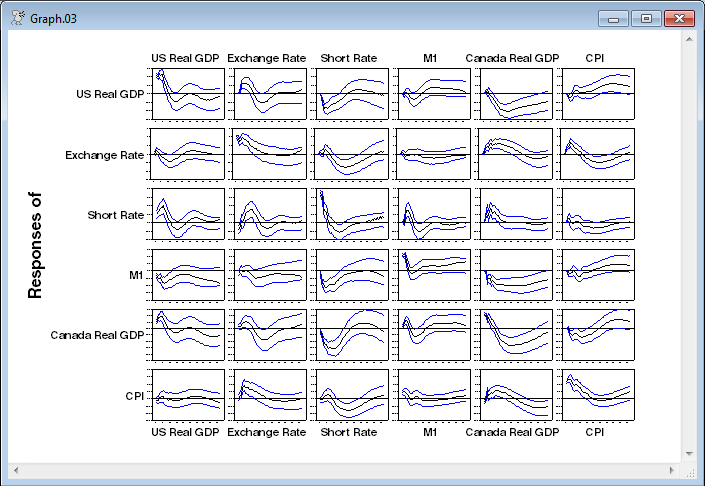
@MONTEVAR does a standard set of IRF confidence bands—it does 16%-84% lower and upper bounds, which are “robust” versions of roughly one-standard error bands. This generates a six by six table of graphs (like @VARIRF with PAGE=ALL), which whjile a bit crowded, is more useful in this form (with confidence bands), since you can tell at a glance which ones are small enough (relative to their bounds) to be ignored.

@montevar(draws=4000,model=canmodel,$

shocks=implabel,varlabels=implabel)

The remainder of the program computes and generates specialized graphs of the impulse responses (in case the standard procedures don't do what you want). The first step is to compute the full block of IRF’s. These go into the RECT[SERIES] called IMPBLK. IMPBLK(i,j) is the response of variable i to a shock in j. IMPULSE with the CV option does Cholesky shocks.

declare rect[series] impblk(neqn,neqn)

declare vect[series] scaled(neqn)

impulse(model=canmodel,result=impblk,noprint,$

steps=nsteps,cv=%sigma)

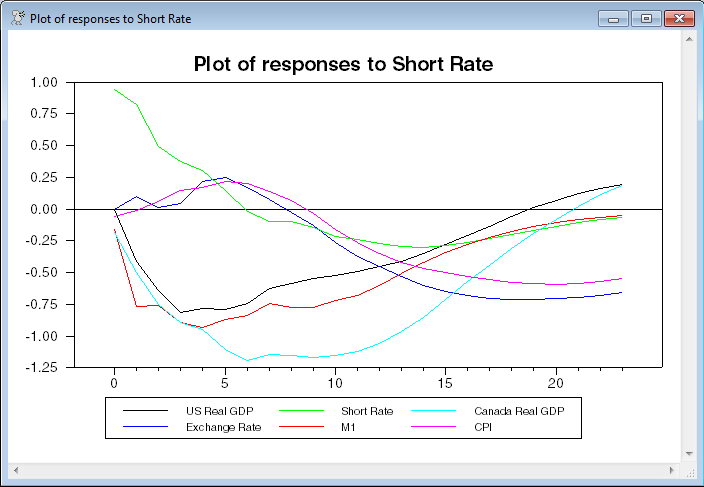
The first loop plots the responses of all series to a single shock. (Basically, this does the same as @VARIRF with PAGE=BYSHOCKS). The response of a series is normalized by dividing by its innovation variance. This allows all the responses to a shock to be plotted (in a reasonable way) on a single scale. Note that these graphs get a bit hard to read with more than five or six variables. The GRAPH uses the NUMBER=0 option to handle the horizontal axis labeling, since that’s the standard way to label IRF’s.

do i=1,neqn

compute header="Plot of responses to "+implabel(i)

do j=1,neqn

set scaled(j) = (impblk(j,i))/sqrt(%sigma(j,j))

end do j

graph(header=header,key=below,klabels=implabel,$

number=0,series=scaled) neqn

end do i

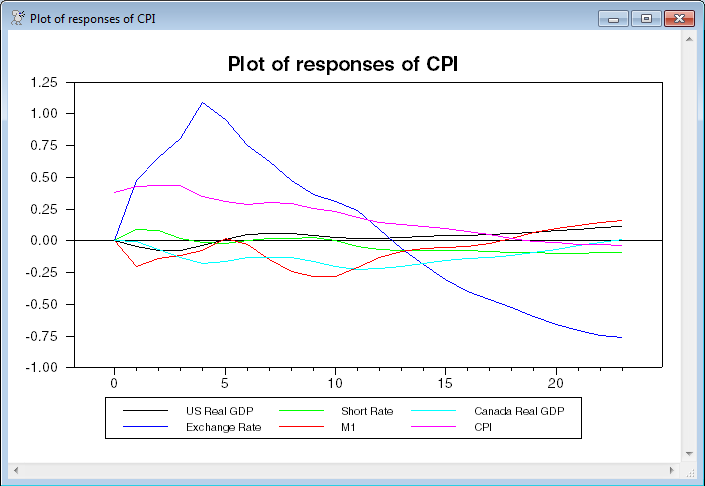
The second loop graphs the responses of a variable to all shocks (@VARIRF with PAGE=BYVARIABLES). These don’t have to be normalized, since the appropriate size of the shocks is determined by the estimates.

do i=1,neqn

compute header="Plot of responses of "+implabel(i)

graph(header=header,key=below,klabels=implabel,number=0,$

series=%scol(impblk,i)) neqn

end do i

A common question has been how to set up a Cholesky or other calculated shock to have a specific impact on a variable—most commonly, a standard size interest rate shock. In this model, the impact of the interest rate shock on itself is .56522. In order to make that (say) -1 while keeping the same “shape” we need to divide by the .56522 (though we will use the program to handle that) and multiply by -1. You could do the standard shocks and rescale after the fact, but it’s easier to just rescale the shock. Both methods are equivalent because of the linearity of the irf’s.

The following takes the Cholesky factor of %SIGMA and extracts the interest rate shock (shock number 3, since it’s the third series in the model). It then rescales it by multiplying by -1 and dividing by the 3rd element (which would be the impact on the interest rate, again, as the third variable).

compute factor=%decomp(%sigma)

compute [vector] rshock=%xcol(factor,3)

compute rshock=-1.0*rshock/rshock(3)

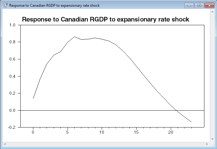
This uses IMPULSE with the SHOCK option to input just the one shock, putting the results in TO_R and graphs the response of Canadian RGDP (the fifth variable in the model). Note that TO_R is still a RECT[SERIES] even though there is just one shock, so you need the (5,1) subscripts to get the response.

impulse(model=canmodel,shock=rshock,steps=nsteps,$

results=to_r,noprint)

graph(number=0,header=$

"Response to Canadian RGDP to expansionary rate shock") 1

# to_r(5,1)

You need to be careful when doing this type of rescaling as it breaks the natural scale that the model has provided. It isn’t recommended that you do this unless this is the only one shock of interest.

Full Program

open data oecdsample.rat
calendar(q) 1981
data(format=rats) 1981:1 2006:4 can3mthpcp canexpgdpchs canexpgdpds $
canm1s canusxsr usaexpgdpch
*
* Scaling the log series by 100 gives the responses a more natural scale.
*
set logcangdp = 100.0*log(canexpgdpchs)
set logcandefl = 100.0*log(canexpgdpds)
set logcanm1   = 100.0*log(canm1s)
set logusagdp = 100.0*log(usaexpgdpch)
set logexrate = 100.0*log(canusxsr)
*
*************************************************************************
*
* The only lines that need to be changed are the ones tagged with ;*<<<<<<
*
compute nlags = 5                                               ;*<<<<<<
compute nsteps = 24                                              ;*<<<<<<
*
system(model=canmodel)
variables logusagdp logexrate can3mthpcp logcanm1 logcangdp logcandefl   ;*<<<<<<<<
lags 1 to nlags
det constant
end(system)
*
* To help create publication-quality graphs, this sets longer labels for
* the series. These are used both in graph headers and key labels.
*
compute [vect[strings]] implabel=|| $                                    ;* <<<<<<
"US Real GDP",$
"Exchange Rate",$
"Short Rate",$
"M1",$
"Canada Real GDP",$
"CPI"||

estimate(noprint)
compute neqn=%nvar
*
* The procedure @VARIRF does the graphs shown below without the extra
* programming. You can choose the graph pages to be organized by shocks
* or by variables.
*
@VARIRF(model=canmodel,steps=nsteps,$
varlabels=implabel,page=byshocks)
@VARIRF(model=canmodel,steps=nsteps,$
varlabels=implabel,page=byvariables)
*
* @MONTEVAR is a simple procedure for doing a standard set of graphs
* with error bands. If you need different formatting on the graphs, use
* a combination of @MCVARDoDraws and @MCGraphIRF (or even more flexibly,
* @MCProcessIRF combined with custom graphs).
*
@montevar(draws=4000,model=canmodel,$
   shocks=implabel,varlabels=implabel,footer="Responses with MC error bands")
*
declare rect[series] impblk(neqn,neqn)
declare vect[series] scaled(neqn)
*
* This computes the full set of impulse responses, which are in the
* series in IMPBLK. IMPBLK(i,j) is the response of variable i to a shock
* in j.
*
impulse(model=canmodel,result=impblk,noprint,$
steps=nsteps,cv=%sigma)
*
* This loop plots the responses of all series to a single series. The
* response of a series is normalized by dividing by its innovation
* variance. This allows all the responses to a shock to be plotted on a
* single scale. Note that these graphs get a bit hard to read with more
* than five or six variables.
*
do i=1,neqn
compute header="Plot of responses to "+implabel(i)
do j=1,neqn
     set scaled(j) = (impblk(j,i))/sqrt(%sigma(j,j))
end do j
graph(header=header,key=below,klabels=implabel,$
    number=0,series=scaled) neqn
end do i
*
* And this loop graphs the responses of a variable to all shocks. These
* don't have to be normalized.
*
do i=1,neqn
compute header="Plot of responses of "+implabel(i)
graph(header=header,key=below,klabels=implabel,number=0,$
     series=%scol(impblk,i)) neqn
end do i
*
* This is specific to this model, as it is set up.
* Normalize interest rate shock to -1.0 impact on itself.
*
compute factor=%decomp(%sigma)
compute [vector] rshock=%xcol(factor,3)
compute rshock=-1.0*rshock/rshock(3)
impulse(model=canmodel,shock=rshock,steps=nsteps,$
   results=to_r,noprint)
graph(number=0,header=$
   "Response of Canadian RGDP to expansionary rate shock") 1
# to_r(5,1)

Graphs

This is the third of the six "to" graphs generated by @VARIRF. Note that, to make such a graph readable, the responses have been scaled to standard deviations, so you can't easily read off any values, just signs and patterns.

This is the last of the "of" graphs generated by @VARIRF. Unlike the "to" graphs, these are in CPI's natural scale, which, with a 100*log(..) transformation means that the response to the exchange rate shock (blue line) is slightly greater than 1% at step 4.

This is the output from the @MONTEVAR. These are set up so that target variables are in rows and shocks in columns, and the target variable responses are all set to use the same scale so the graphs can easily be compared as you look across a row.

This is the graph generated by shock of size -1 to the interest rate. With the 100 log(..) transformation, you read this as a maximum effect of a roughly .8% increase at steps 6 through 10.