BASICFORECAST.RPF

BASICFORECAST.RPF includes most of the code segments from Forecasting (Introduction). For a single equation (linear) model, it demonstrates static and dynamic forecasting, forecasts with rolling samples, and the use of the @UFOREERRORS and @DMARIANO procedures.

Note well that this is intended to show a variety of techniques, many of which would not necessarily be used together.

The data are monthly on retail sales through 1994, though for much of the analysis, the final year of data are held back with forecasts being made for the year 1994. The first model is simply a linear time trend on the log of the original data:

set logrsales = log(rsales)

set time = t

linreg(define=saleseq) logrsales * 1993:12

# constant time

DEFINE=SALESEQ defines a (linear) EQUATION of that name from the results of the LINREG. SALESEQ will be used in the code that follows to do the forecasts.

The program demonstrates several ways to do the forecasts, some of which aren't recommended, but show a syntax you might see in RATS programs written for earlier versions of the software.

The simplest instruction for forecasting a univariate model like this is UFORECAST:

uforecast(equation=saleseq) logfore 1994:1 1994:12

which produces the series LOGFORE over 1994:1 to 1994:12 using the equation saved in SALESEQ.

FORECAST is a useful instruction when you have a model with more than one equation. It's clumsier than UFORECAST when you have just one.

forecast(from=1994:1,to=1994:12) 1

# saleseq logfore

forecast(steps=12) 1

# saleseq logfore

The SMPL instruction can be used to set the forecast range (and again you might see that in older programs), but we strongly discourage its use:

smpl 1994:1 1994:12

forecast 1

# saleseq logfore

* This turns the SMPL off so it doesn't have unwanted effects.

smpl

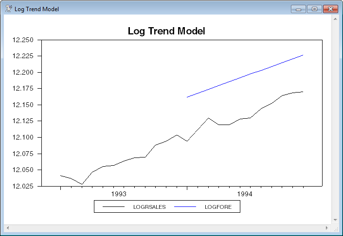
Back to the main line of the example, this uses the recommended instruction for generating the forecasts, then uses a GRAPH instruction to graph the original data (in log form) over the period 1993:1 to 1994:12, along with the forecasts. Note the use of the range parameters on LOGRSALES to control which enteries of the original data are included. If you just put in LOGRSALES without the range, you would get the entire range of LOGRSALES back to 1954:1, so the actual forecast period would only form a small segment of the graph. Choosing a shorter range focuses the graph more on the period of interest.

uforecast(equation=saleseq) logfore 1994:1 1994:12

graph(key=below,header="Log Trend Model") 2

# logrsales 1993:1 1994:12

# logfore

The remainder of the example uses a more realistic model for the data series, with constant, trend and a lagged dependent variable. (The original regression with just a trend has a very low Durbin-Watson, indicating that it does a poor job of dealing with the dynamic behavior of the data).

Rolling Regressions

It's a common task in evaluating the ability of a model to forecast to do "rolling" (sample) regressions to simulate how the model might have worked in real time, where you would typically use all available data through period T to forecast do forecasts from T+1 to T+h (where h is the forecast horizon of interest), but would not have data from the forecast period itself. Thus to do a series of simulated "ex ante" forecasts, you need to change the range of the regression. (Note that this is only simulating how the model would have worked because the current data series may have been revised from the historical data).

The first example does rolling regressions with a fixed start period and an end period which increases over the interval where we are doing the forecasts. The end of samples are 1991:12 through 1994:11. It does one forecast step after each estimation period, putting the results into the series RHAT.

clear rhat

do regend=1991:12,1994:11

linreg(noprint) logrsales * regend

# constant time logrsales{1}

uforecast rhat regend+1 regend+1

end do

The * in the start parameter on the LINREG means that the sample for that starts at the earliest possible period given the data and the model. Here, because the model requires one lag of LOGRSALES, it will be entry 2 (that is, 1954:2). Note that this uses the NOPRINT option on the LINREG so you won't get output from 36 regressions. In general, you should only put NOPRINT options on once you are sure that this is doing what you want.

UFORECAST, by default, does its forecasts using the most recently estimated regression, so it isn't necessary in this case (and in the examples above) to define and input an EQUATION to it.

This next segment does a rolling regression but with a moving 60 period (five year) estimation window. The only change to the LINREG is to use REGEND-59 as the start parameter. In addition to the one-step forecasts (again going into RHAT, so this is overwriting the previous forecasts—in practice, you would pick either the fixed start samples or the rolling samples, but not both). In addition to saving the forecasts, this also saves the rolling coefficient estimates into COEF1, COEF2 and COEF3.

clear rhat coef1 coef2 coef3

do regend=1991:12,1994:11

linreg(noprint) logrsales regend-59 regend

# constant time logrsales{1}

compute coef1(regend) = %beta(1)

compute coef2(regend) = %beta(2)

compute coef3(regend) = %beta(3)

uforecast rhat regend+1 regend+1

end do

The next segment does a similar 60-period rolling regression, but does 12-step-ahead (dynamic) forecasts. Multiple step dynamic forecasts for a model with lagged dependent variables (like this one) feed the early step forecasts into the calculations of the later steps rather than going back to the observed data. Dynamic forecasts are the default for UFORECAST. This saves the 12-step forecasts into the series RHAT12. Note that the forecast 12 periods ahead from REGEND will be in entry REGEND+12 of RHAT. This cuts the set of regressions down to end with 1993:12 to allow for 12 forecast periods.

clear rhat rhat12

do regend=1991:12,1993:12

linreg(noprint) logrsales regend-59 regend

# constant time logrsales{1}

uforecast rhat regend+1 regend+12

compute rhat12(regend+12)=rhat(regend+12)

end do

This does the same thing as above, but uses FORECAST with the SKIPSAVE option (SKIPSAVE=11 tells FORECAST to not save the first 11 forecasts, thus only the 12th.)

clear rhat12

do regend=1991:1,1993:12

linreg(define=foreeq,noprint) logrsales regend-59 regend

# constant time logrsales{1}

forecast(skipsave=11,steps=12)

# foreeq rhat12

end do

Returning the original simple model, this uses PRJ to a series of one-step in-sample forecasts. If you use PRJ to compute forecasts (it can only do static forecasts), you can use the STDERRS option to produce a series of the standard errors of projection. This estimates the model through 1993:12, does forecasts through 1994:12, and creates series FORE, UPPER and LOWER with forecasts and upper and lower bounds (using 1.96 standard errors) transformed back into levels from logs.

linreg(define=saleseq) logrsales * 1993:12

# constant time

prj(stderrs=stderrs) logfore 1994:1 1994:12

set upper 1994:1 1994:12 = exp(logfore+1.96*stderrs)

set lower 1994:1 1994:12 = exp(logfore-1.96*stderrs)

set fore 1994:1 1994:12 = exp(logfore)

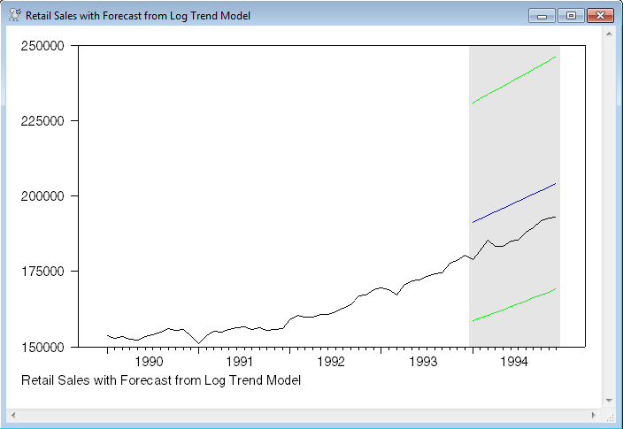
This next graphs the forecasts, with the error bounds, with five years of prior actual data, adding shading over the forecast range. The shading is done using

set y1994 = %year(t)==1994

which creates a dummy variable which is 1 for entries where the year is 1994 (and 0's elsewhere). This is added to the GRAPH using the SHADING option:

graph(shading=y1994,footer=$

"Retail Sales with Forecast from Log Trend Model") 4

# rsales 1990:1 1994:12

# fore

# upper / 3

# lower / 3

Forecast Error Analysis

The following does rolling sample estimates and forecasts one period out for each period from 1992:1 to 1994:12. It then uses @UFOREERRORS to analyze the forecast errors (which it does by comparing the forecasts to the actual data). Note that this has to be done in-sample, since it needs the actual data for comparison.

clear rhat

do fstart=1992:1,1994:12

linreg(noprint) logrsales * fstart-1

# constant time logrsales{1}

uforecast rhat fstart fstart

end do

@uforeerrors logrsales rhat 1992:1 1994:12

The most useful statistics in the @UFOREERRORS output are usually the Root Mean Square Error (RMSE) and the Root Mean Square Percentage Error. Here, because the series being forecast is already in logs, the RMSE would be the one chosen. With the data being straight logs (sometimes 100*log's are used, which would multiply this by 100 and make it easier to read off percentages), .00787 means the RMSE is a bit less than 1% (0.787% to be more precise).

The final calculation in the example is to do a Diebold-Mariano test using @DMARIANO, comparing the forecasts just made with "naive" forecasts that just use the previous data point. Since the series is trending, we would expect forecasts which include the trend would do better, and that is what the output shows.

set naive 1992:1 1994:12 = logrsales{1}

@dmariano logrsales naive rhat

Full Program

cal(m) 1954:1
open data rsales.dat
data(format=prn,org=columns) 1954:1 1994:12
*
* Data on the file run through 1994, but the final year is "held back"
* from the forecasting exercises.
*
graph(footer="Retail Sales")
# rsales
*
set logrsales = log(rsales)
set time = t
*
linreg(define=saleseq) logrsales * 1993:12
# constant time
***********************************************************************
*
* Alternative ways of getting forecasts of log sales from 1994:1 to
* 1994:12.
*
uforecast(equation=saleseq) logfore 1994:1 1994:12
*
forecast(from=1994:1,to=1994:12) 1
# saleseq logfore
*
forecast(steps=12) 1
# saleseq logfore
*
* The use of SMPL to set the range works, but isn't recommended.
*
smpl 1994:1 1994:12
forecast 1
# saleseq logfore
*
* This turns the SMPL off so it doesn't have unwanted effects.
*
smpl
*
***********************************************************************
uforecast(equation=saleseq) logfore 1994:1 1994:12
graph(key=below,header="Log Trend Model") 2
# logrsales 1993:1 1994:12
# logfore
*
* Forecast with rolling regression with fixed front end
*
clear rhat
do regend=1991:12,1994:11
   linreg(noprint) logrsales * regend
   # constant time logrsales{1}
   uforecast rhat regend+1 regend+1
end do
*
* Forecast with rolling regression with moving 60 period window
*
clear rhat coef1 coef2 coef3
do regend=1991:12,1994:11
   linreg(noprint) logrsales regend-59 regend
   # constant time logrsales{1}
   compute coef1(regend) = %beta(1)
   compute coef2(regend) = %beta(2)
   compute coef3(regend) = %beta(3)
   uforecast rhat regend+1 regend+1
end do
*
* Rolling regression, saving the 12 step out forecasts
* Copying information out to separate series
*
clear rhat rhat12
do regend=1991:12,1993:12
   linreg(noprint) logrsales regend-59 regend
   # constant time logrsales{1}
   uforecast rhat regend+1 regend+12
   compute rhat12(regend+12)=rhat(regend+12)
end do
*
* Same thing but using FORECAST with SKIPSAVE
*
clear rhat12
do regend=1991:1,1993:12
   linreg(define=foreeq,noprint) logrsales regend-59 regend
   # constant time logrsales{1}
   forecast(skip=11,steps=12)
   # foreeq rhat12
end do
*
* Use of PRJ with STDERRS
*
linreg(define=saleseq) logrsales * 1993:12
# constant time
prj(stderrs=stderrs) logfore 1994:1 1994:12
set fore 1994:1 1994:12 = exp(logfore)
set upper 1994:1 1994:12 = exp(logfore+1.96*stderrs)
set lower 1994:1 1994:12 = exp(logfore-1.96*stderrs)
*
* Create series which is 1's where we want shading.
*
set y1994 = %year(t)==1994
*
* Graph forecasts, upper and lower bounds and several years of actual
* data, with shading over the forecast range.
*
graph(shading=y1994,footer=$
"Retail Sales with Forecast from Log Trend Model") 4
# rsales 1990:1 1994:12
# fore
# upper / 3
# lower / 3
*
* Forecast error analysis
* Do forecasts for 1992:1 through 1994:12, using data through the period
* prior in each case.
*
clear rhat
do fstart=1992:1,1994:12
   linreg(noprint) logrsales * fstart-1
   # constant time logrsales{1}
   uforecast rhat fstart fstart
end do
@uforeerrors logrsales rhat 1992:1 1994:12
*
* Diebold-Mariano test
*
set naive 1992:1 1994:12 = logrsales{1}
@dmariano logrsales naive rhat

Output

Linear Regression - Estimation by Least Squares

Dependent Variable LOGRSALES

Monthly Data From 1954:01 To 1993:12

Usable Observations 480

Degrees of Freedom 478

Centered R^2 0.9864741

R-Bar^2 0.9864458

Uncentered R^2 0.9999219

Mean of Dependent Variable 10.750051618

Std Error of Dependent Variable 0.819886278

Standard Error of Estimate 0.095453187

Sum of Squared Residuals 4.3552066221

Regression F(1,478) 34861.6206

Significance Level of F 0.0000000

Log Likelihood 447.4889

Durbin-Watson Statistic 0.0185

Variable Coeff Std Error T-Stat Signif

************************************************************************************

1. Constant 9.3381351301 0.0087272768 1069.99415 0.00000000

2. TIME 0.0058707546 0.0000314427 186.71267 0.00000000

Linear Regression - Estimation by Least Squares

Dependent Variable LOGRSALES

Monthly Data From 1954:01 To 1993:12

Usable Observations 480

Degrees of Freedom 478

Centered R^2 0.9864741

R-Bar^2 0.9864458

Uncentered R^2 0.9999219

Mean of Dependent Variable 10.750051618

Std Error of Dependent Variable 0.819886278

Standard Error of Estimate 0.095453187

Sum of Squared Residuals 4.3552066221

Regression F(1,478) 34861.6206

Significance Level of F 0.0000000

Log Likelihood 447.4889

Durbin-Watson Statistic 0.0185

Variable Coeff Std Error T-Stat Signif

************************************************************************************

1. Constant 9.3381351301 0.0087272768 1069.99415 0.00000000

2. TIME 0.0058707546 0.0000314427 186.71267 0.00000000

Forecast Analysis for LOGRSALES

From 1992:01 to 1994:12

Mean Error -0.0010513

Mean Absolute Error 0.0063035

Root Mean Square Error 0.0078721

Mean Square Error 0.000062

Theil's U 0.804946

Mean Pct Error -0.000087

Mean Abs Pct Error 0.000522

Root Mean Square Pct Error 0.000652

Theil's Relative U 0.804599

Diebold-Mariano Forecast Comparison Test

Forecasts of LOGRSALES over 1992:01 to 1994:12

Forecast MSE Test Stat P(DM>x)

NAIVE 0.00009564 1.8669 0.03096

RHAT 0.00006197 -1.8669 0.96904

Graphs