BOOTVECM.RPF

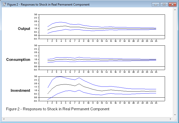
BOOTVECM.RPF does a parametric bootstrap (to get error bands for an IRF) of a VECM with known cointegrating vector. The model used is from King, Plosser, Stock and Watson(1991).

Full Program

*
* This does a parametric bootstrap (to get error bands for an IRF) of a
* VECM with known cointegrating vector. The model used is from King,
* Plosser, Stock and Watson(1991), "Stochastic Trends and Economic
* Fluctuations", AER, vol 81, pp 819-840.
*
compute ndraws=500
compute nvar =3
compute nstep =25
*
open data kpswdata.rat
calendar(q) 1947
data(format=rats) 1947:1 1988:4 c in y mp dp r
*
equation(coeffs=||1.0,-1.0||) covery
# c y
equation(coeffs=||1.0,-1.0||) iovery
# in y
*
system(model=vecmmodel)
variables y c in
lags 1 to 9
det constant
ect covery iovery
end(system)
*
estimate(resids=baseresids)
*
compute basevecm=%modelsubstect(vecmmodel)
*
source varbootsetup.src
source forcedfactor.src
*
dec vect[series] %%VARResample(nvar)
do i=1,nvar
   set %%VARResample(i) = %modeldepvars(basevecm)(i){0}
end do i
equation(coeffs=||1.0,-1.0||) coveryboot
# %%VARResample(2) %%VARResample(1)
equation(coeffs=||1.0,-1.0||) ioveryboot
# %%VARResample(3) %%VARResample(1)
*
system(model=bootvecm)
variables %%VARResample
lags 1 to 9
det constant
ect coveryboot ioveryboot
end(system)
*
* To isolate the balanced growth shock
*
compute atilde=||1.0|1.0|1.0||
*
* Bookkeeping series for the IRF for the balanced growth shock and the
* error decomposition percentages.
*
dec rect[series] %%responses(nstep,nvar)
dec rect[series] errors(nstep,nvar)
do i=1,nstep
   do j=1,nvar
      set %%responses(i,j) 1 ndraws = 0.0
      set errors(i,j) 1 ndraws    = 0.0
   end do j
end do i
*
infobox(action=define,progress,lower=1,upper=ndraws) "Bootstrapping"
do draws = 1,ndraws
   @VARBootDraw(model=basevecm,resids=baseresids) %regstart() %regend()
   estimate(noprint)
   impulse(model=bootvecm,factor=%identity(3),results=baseimp,noprint,steps=500)
   compute lrsum=%xt(baseimp,500)
   *
   compute d=inv(%innerxx(atilde))*tr(atilde)*lrsum
   @forcedfactor(force=row) %sigma d f
   compute lrfactor=lrsum*f
   impulse(noprint,model=bootvecm,factor=f/lrfactor(1,1),results=impulses,steps=25)
   *
   * Store the impulse responses. In this case, we're only interested in
   * the responses to the first shock.
   *
   do i=1,nstep
      do j=1,nvar
         set %%responses(i,j) draws draws = impulses(j,1)(i)
      end do i
   end do i
   *
   * Store the decomposition of variance. Again, we're only interested
   * in the fraction explained by the first shock.
   *
   errors(noprint,model=bootvecm,factor=f,results=decvar,steps=25)
   do i=1,nstep
      do j=1,nvar
         set errors(i,j) draws draws = decvar(j,1)(i)
      end do j
   end do i
   infobox(current=draws)
end do draws
infobox(action=remove)
*
report(action=define)
report(atrow=1,atcol=1,tocol=4,span) "Fraction of the forecast-error variance"
report(atrow=2,atcol=1,tocol=4,span) "attributed to the real permanent shock"
report(atrow=3,atcol=1,align=center) "Horizon" "y" "c" "i"
compute row=1
dofor horizon = 1 4 8 12 16 20 24
   compute row=row+3
   report(atrow=row,atcol=1) horizon
   do j=1,nvar
      stats(noprint) errors(horizon,j) 1 ndraws
      report(atrow=row,atcol=j+1) %mean
      report(atrow=row+1,atcol=j+1,special=parens) sqrt(%variance)
   end do j
end do horizon
report(action=format,picture="*.##",atrow=4,align=decimal)
report(action=show)
*
*
dec vect[series] mid(nvar) upper(nvar) lower(nvar)
do j=1,nvar
   do i=1,nstep
      sstats(mean) 1 ndraws %%responses(i,j)>>first %%responses(i,j)^2>>second
      compute stddev=sqrt(second-first^2)
      set mid(j)   i i = first
      set upper(j) i i = first+stddev
      set lower(j) i i = first-stddev
   end do i
end do j
*
table(noprint) 1 nstep upper lower
*
spgraph(vfields=nvar,ylabels=||"Output","Consumption","Investment"||,$
footer="Figure 2 - Responses to Shock in Real Permanent Component")
do j=1,nvar
   graph(max=%maximum,min=%minimum,nodates) 3
   # mid(j)
   # upper(j) / 2
   # lower(j) / 2
end do j
spgraph(done)

Output

VAR/System - Estimation by Cointegrated Least Squares

Quarterly Data From 1949:02 To 1988:04

Usable Observations 159

Dependent Variable Y

Mean of Dependent Variable 0.0044331132

Std Error of Dependent Variable 0.0137793141

Standard Error of Estimate 0.0120057747

Sum of Squared Residuals 0.0190262987

Durbin-Watson Statistic 1.9424

Variable Coeff Std Error T-Stat Signif

************************************************************************************

1. D_Y{1} 0.047429300 0.122965755 0.38571 0.70033129

2. D_Y{2} -0.012323764 0.126730017 -0.09724 0.92267994

3. D_Y{3} -0.104273993 0.126064403 -0.82715 0.40964563

4. D_Y{4} -0.198319377 0.131009902 -1.51377 0.13247392

5. D_Y{5} -0.122728992 0.130421869 -0.94102 0.34841587

6. D_Y{6} 0.020049919 0.131106809 0.15293 0.87868848

7. D_Y{7} -0.022636669 0.129011123 -0.17546 0.86098477

8. D_Y{8} 0.105349100 0.122939910 0.85692 0.39304469

9. D_C{1} 0.298015644 0.164671728 1.80976 0.07260878

10. D_C{2} 0.085246112 0.166460224 0.51211 0.60942908

11. D_C{3} 0.067202023 0.166092563 0.40461 0.68642213

12. D_C{4} 0.259950290 0.166805226 1.55841 0.12153138

13. D_C{5} 0.001430640 0.170613749 0.00839 0.99332227

14. D_C{6} 0.070068633 0.170344568 0.41133 0.68149419

15. D_C{7} 0.151681055 0.168650291 0.89938 0.37008693

16. D_C{8} -0.318507940 0.163076442 -1.95312 0.05292090

17. D_IN{1} 0.123881211 0.061687618 2.00820 0.04666253

18. D_IN{2} 0.009222750 0.061826276 0.14917 0.88164556

19. D_IN{3} -0.014940205 0.061992272 -0.24100 0.80992821

20. D_IN{4} 0.012472142 0.063266782 0.19714 0.84402456

21. D_IN{5} 0.018316131 0.062264946 0.29416 0.76909435

22. D_IN{6} 0.002441596 0.059253697 0.04121 0.96719410

23. D_IN{7} -0.020226022 0.058075103 -0.34827 0.72818959

24. D_IN{8} -0.059550855 0.055247789 -1.07789 0.28305019

25. Constant 0.072407668 0.064538071 1.12194 0.26392584

26. EC1{1} 0.098691320 0.054816898 1.80038 0.07408397

27. EC2{1} 0.029635937 0.038292048 0.77394 0.44034729

Dependent Variable C

Mean of Dependent Variable 0.0047516415

Std Error of Dependent Variable 0.0081083615

Standard Error of Estimate 0.0074663470

Sum of Squared Residuals 0.0073585166

Durbin-Watson Statistic 1.9402

Variable Coeff Std Error T-Stat Signif

************************************************************************************

1. D_Y{1} 0.085577118 0.076471949 1.11907 0.26514447

2. D_Y{2} -0.014484099 0.078812930 -0.18378 0.85446946

3. D_Y{3} -0.239662718 0.078398987 -3.05696 0.00270703

4. D_Y{4} -0.115555460 0.081474575 -1.41830 0.15845954

5. D_Y{5} -0.151264533 0.081108879 -1.86496 0.06440791

6. D_Y{6} 0.055668642 0.081534841 0.68276 0.49595568

7. D_Y{7} -0.042588387 0.080231542 -0.53082 0.59643653

8. D_Y{8} 0.069060761 0.076455876 0.90328 0.36802485

9. D_C{1} -0.067970562 0.102408740 -0.66372 0.50802815

10. D_C{2} 0.173666464 0.103520999 1.67760 0.09579222

11. D_C{3} 0.157331252 0.103292352 1.52316 0.13010969

12. D_C{4} 0.115348557 0.103735555 1.11195 0.26818154

13. D_C{5} 0.059460705 0.106104061 0.56040 0.57615660

14. D_C{6} -0.024408985 0.105936658 -0.23041 0.81812903

15. D_C{7} 0.205110090 0.104882993 1.95561 0.05262362

16. D_C{8} -0.139637889 0.101416638 -1.37687 0.17088203

17. D_IN{1} 0.025239645 0.038363302 0.65791 0.51174093

18. D_IN{2} 0.015630006 0.038449533 0.40651 0.68502839

19. D_IN{3} 0.083659079 0.038552765 2.16999 0.03179777

20. D_IN{4} 0.025406131 0.039345378 0.64572 0.51958108

21. D_IN{5} 0.013943309 0.038722340 0.36008 0.71935954

22. D_IN{6} 0.010538158 0.036849656 0.28598 0.77534396

23. D_IN{7} -0.003811119 0.036116693 -0.10552 0.91612151

24. D_IN{8} -0.019607987 0.034358396 -0.57069 0.56918016

25. Constant -0.057089740 0.040135988 -1.42241 0.15726672

26. EC1{1} -0.012372023 0.034090427 -0.36292 0.71724676

27. EC2{1} -0.036463459 0.023813683 -1.53120 0.12811361

Dependent Variable IN

Mean of Dependent Variable 0.0046512327

Std Error of Dependent Variable 0.0283198006

Standard Error of Estimate 0.0223188716

Sum of Squared Residuals 0.0657534282

Durbin-Watson Statistic 1.9954

Variable Coeff Std Error T-Stat Signif

************************************************************************************

1. D_Y{1} 0.622798781 0.228594736 2.72447 0.00731335

2. D_Y{2} 0.087807300 0.235592541 0.37271 0.70996332

3. D_Y{3} -0.225447265 0.234355158 -0.96199 0.33781367

4. D_Y{4} -0.427267578 0.243548897 -1.75434 0.08169284

5. D_Y{5} -0.260411190 0.242455737 -1.07406 0.28475677

6. D_Y{6} -0.165996824 0.243729048 -0.68107 0.49701952

7. D_Y{7} -0.127641129 0.239833144 -0.53221 0.59547658

8. D_Y{8} -0.015034652 0.228546690 -0.06578 0.94764954

9. D_C{1} 0.080535956 0.306126614 0.26308 0.79289870

10. D_C{2} 0.087479540 0.309451448 0.28269 0.77785553

11. D_C{3} 0.167747190 0.308767962 0.54328 0.58785390

12. D_C{4} 0.502290017 0.310092812 1.61981 0.10766076

13. D_C{5} 0.360884036 0.317172898 1.13781 0.25725884

14. D_C{6} 0.266393351 0.316672488 0.84123 0.40174230

15. D_C{7} 0.618572648 0.313522807 1.97297 0.05058777

16. D_C{8} -0.462079871 0.303160960 -1.52421 0.12984945

17. D_IN{1} 0.292004478 0.114677982 2.54630 0.01203570

18. D_IN{2} -0.048678360 0.114935749 -0.42353 0.67260031

19. D_IN{3} 0.106663865 0.115244338 0.92555 0.35637131

20. D_IN{4} 0.023413844 0.117613667 0.19907 0.84251103

21. D_IN{5} 0.023712361 0.115751243 0.20486 0.83800002

22. D_IN{6} 0.186960805 0.110153297 1.69728 0.09200062

23. D_IN{7} -0.048263782 0.107962277 -0.44704 0.65557665

24. D_IN{8} 0.048688352 0.102706267 0.47405 0.63624436

25. Constant -0.276351728 0.119977008 -2.30337 0.02282108

26. EC1{1} 0.153536085 0.101905236 1.50666 0.13428842

27. EC2{1} -0.195691048 0.071185352 -2.74904 0.00681486

Fraction of the forecast-error variance

attributed to the real permanent shock

Horizon y c i

1 0.37 0.74 0.13

(0.28) (0.19) (0.15)

4 0.46 0.75 0.27

(0.28) (0.17) (0.21)

8 0.55 0.74 0.35

(0.23) (0.16) (0.18)

12 0.61 0.77 0.39

(0.20) (0.15) (0.17)

16 0.64 0.80 0.41

(0.18) (0.13) (0.16)

20 0.67 0.82 0.42

(0.17) (0.11) (0.16)

24 0.70 0.84 0.44

(0.17) (0.10) (0.16)

Graph