BOOTVAR.RPF

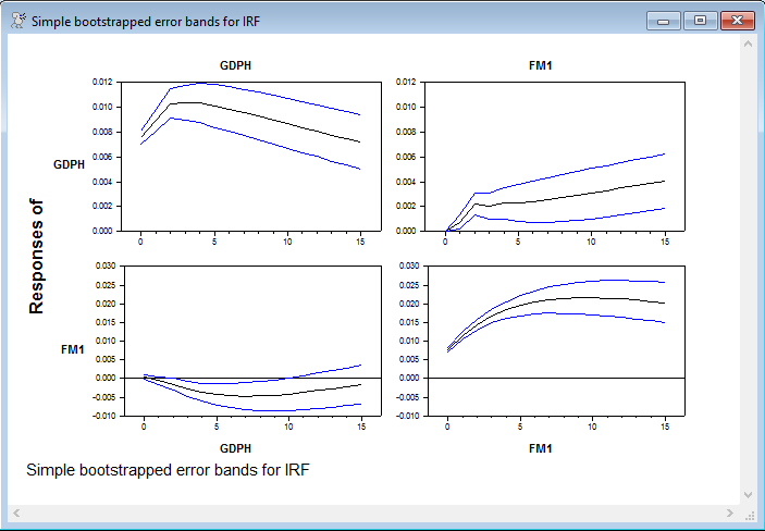
BOOTVAR.RPF is an example of simple bootstrapping to get error bands for the impulse response functions for a VAR. Note that this does not do the bias-corrected bootstrap-in-bootstrap methods proposed by Kilian(1998). There's a separate replication program for that.

Full Program

compute lags=4 ;*Number of lags

compute nvar=2 ;*Number of variables

compute nstep=16 ;*Number of response steps

compute ndraws=2500 ;*Number of draws

open data haversample.rat

calendar(q) 1959

data(format=rats) 1959:1 2006:4 fm1 gdph

log gdph

log fm1

******************************************************************

* Set up the system

dec vect[series] udraws(nvar) resids(nvar) resample(nvar)

dec vect[equation] eqsample(nvar) eqbase(nvar)

system(model=varmodel)

variables gdph fm1

lags 1 to lags

det constant

end(system)

estimate(resids=resids)

* Save the estimation range

compute bstart=%regstart(),bend=%regend()

* Set up the parallel system for the resampled data

@VARBootSetup(model=varmodel) bootvar

* For saving the generated responses

declare vect[rect] %%responses(ndraws)

infobox(action=define,progress,lower=1,upper=ndraws) "Bootstrap Simulations"

do draw=1,ndraws

infobox(current=draw)

* Draw the new data

@VARBootDraw(model=varmodel,resids=resids) bstart bend

* Estimate the VAR on the bootstrapped data

estimate(model=bootvar,noprint) bstart bend

* Compute and save the IRF's

impulse(noprint,model=bootvar,cv=%sigma,flatten=%%responses(draw),steps=nstep)

end do draw

infobox(action=remove)

@MCGraphIRF(model=varmodel,page=all,footer="Simple bootstrapped error bands for IRF")

Output

(These are just the results of the original least squares estimates).

VAR/System - Estimation by Least Squares

Quarterly Data From 1960:01 To 2006:04

Usable Observations 188

Dependent Variable GDPH

Mean of Dependent Variable 8.6324850619

Std Error of Dependent Variable 0.4316368147

Standard Error of Estimate 0.0079905839

Sum of Squared Residuals 0.0114290481

Durbin-Watson Statistic 1.9550

Variable Coeff Std Error T-Stat Signif

************************************************************************************

1. GDPH{1} 1.197873769 0.073449800 16.30874 0.00000000

2. GDPH{2} -0.030449933 0.114752060 -0.26535 0.79104201

3. GDPH{3} -0.163097143 0.112846167 -1.44531 0.15012062

4. GDPH{4} -0.017530569 0.072609443 -0.24144 0.80949319

5. FM1{1} 0.095748085 0.071755895 1.33436 0.18378139

6. FM1{2} 0.022935583 0.130475231 0.17578 0.86066159

7. FM1{3} -0.288056534 0.130878837 -2.20094 0.02901963

8. FM1{4} 0.175959556 0.072164873 2.43830 0.01573335

9. Constant 0.077885100 0.039882091 1.95288 0.05239257

F-Tests, Dependent Variable GDPH

Variable F-Statistic Signif

*******************************************************

GDPH 4372.9597 0.0000000

FM1 2.4499 0.0478566

Dependent Variable FM1

Mean of Dependent Variable 6.1687053805

Std Error of Dependent Variable 0.7805932208

Standard Error of Estimate 0.0081970360

Sum of Squared Residuals 0.0120272606

Durbin-Watson Statistic 2.0063

Variable Coeff Std Error T-Stat Signif

************************************************************************************

1. GDPH{1} -0.160034568 0.075347518 -2.12395 0.03504738

2. GDPH{2} 0.113867528 0.117716901 0.96730 0.33469933

3. GDPH{3} 0.006340586 0.115761766 0.05477 0.95638062

4. GDPH{4} 0.044662752 0.074485448 0.59962 0.54951966

5. FM1{1} 1.514081794 0.073609847 20.56901 0.00000000

6. FM1{2} -0.352299006 0.133846311 -2.63212 0.00922663

7. FM1{3} -0.091614320 0.134260344 -0.68236 0.49589138

8. FM1{4} -0.073995043 0.074029392 -0.99954 0.31888438

9. Constant -0.013065248 0.040912522 -0.31935 0.74983657

F-Tests, Dependent Variable FM1

Variable F-Statistic Signif

*******************************************************

GDPH 2.0141 0.0943924

FM1 13946.5414 0.0000000

Graphs