CONDITION.RPF

CONDITION.RPF demonstrates conditional forecasting, using the same data set as in IMPULSES.RPF and several other examples. It computes forecasts conditional on 5% year over year growth in the US GDP. This type of constraint is easy to handle because US GDP is in logs.

After the model is set up and estimated, this sets the forecast range

compute fstart=2007:1,fend=2009:4

This uses the @CONDITION procedure to create the conditional forecasts into the series CONDFORE(1) to CONDFORE(6). Note that you use the name of the dependent variable on the constraint. The first constraint has LOGUSAGDP at 2007:4 hitting the value of the same series at 2006:4 plus .05 (for 5% year over year growth), and the second has a 10% change over two years to 2008:4.

@condition(model=canmodel,from=fstart,to=fend,results=condfore) 2

# logusagdp 2007:4 logusagdp(2006:4)+.05

# logusagdp 2008:4 logusagdp(2006:4)+.10

The next computes the unconditional forecasts into FORECAST(1) to FORECAST(6).

forecast(model=canmodel,results=forecasts,from=fstart,to=fend)

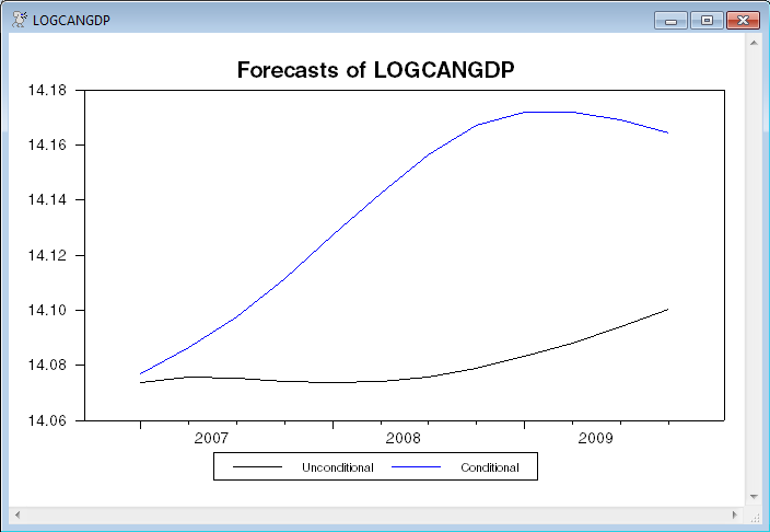
And this graphs the conditional and unconditional forecasts for each of the series.

do i=1,neqn

compute [label] l=%modellabel(canmodel,i)

graph(header="Forecasts of "+l,window=l,$

key=below,klabels=||"Unconditional","Conditional"||) 2

# forecasts(i)

# condfore(i)

end do i

The remainder of the program is more technical. It does a set of 1000 simulations subject to the same constraint. The results of this for the Canadian GDP are analyzed on two graphs. Both of these show the .16 and .84 quantiles of the simulated values: these correspond roughly to one standard error. Because we need a simulated series for each draw, and because we need the full history of the simulations (there are no sufficient statistics for order statistics, so you need all the generated data), the following sets up a SERIES[VECTOR]. At each entry from FSTART to FEND, this will have a 1000-vector with the simulated values for Canadian RGDP.

compute ndraws=1000

dec series[vect] can

gset can fstart fend = %zeros(ndraws,1)

For each draw, this does a simulation subject to the constraints, and saves the simulated values for Canadian RGDP (variable 1 as this model is ordered).

do draw=1,ndraws

@condition(simulate,model=canmodel,from=fstart,to=fend,$

results=simfore) 2

# logusagdp 2007:4 logusagdp(2006:4)+.05

# logusagdp 2008:4 logusagdp(2006:4)+.10

do t=fstart,fend

compute can(t)(draw)=simfore(1)(t)

end do t

end do draw

This computes the 84th and 16th percentiles of the distribution at each point in the forecast range and graphs the unconditional and conditional forecasts (again, the target variable is variable 1 in the model) along with the upper and lower bounds.

set upper fstart fend = %fractiles(can(t),||.84||)(1)

set lower fstart fend = %fractiles(can(t),||.16||)(1)

graph(key=below,$

header="Canadian Real GDP with High Growth of US GDP",$

klabels=||"Unconditional","Conditional","84%ile","16%ile"||) 4

# forecasts(1)

# condfore(1)

# upper / 3

# lower / 3

These transform the various GDP numbers into average (annualized) growth rates from FSTART-1 and does a combined graph.

set fgrowth fstart fend = $

400.0*(forecasts(1)-logcangdp(fstart-1))/(t-fstart+1)

set cgrowth fstart fend = $

400.0*(condfore(1)-logcangdp(fstart-1))/(t-fstart+1)

set ugrowth fstart fend = $

400.0*(upper-logcangdp(fstart-1))/(t-fstart+1)

set lgrowth fstart fend = $

400.0*(lower-logcangdp(fstart-1))/(t-fstart+1)

graph(key=below,$

header="Canadian GDP Average Growth with High Growth of US GDP",$

klabels=||"Unconditional","Conditional","84%ile","16%ile"||) 4

# fgrowth

# cgrowth

# ugrowth / 3

# lgrowth / 3

Full Program

open data oecdsample.rat
calendar(q) 1981
data(format=rats) 1981:1 2006:4 can3mthpcp canexpgdpchs $
   canexpgdpds canm1s canusxsr usaexpgdpch
*
set logcangdp = log(canexpgdpchs)
set logcandefl = log(canexpgdpds)
set logcanm1   = log(canm1s)
set logusagdp = log(usaexpgdpch)
set logexrate = log(canusxsr)
*
system(model=canmodel)
variables logcangdp logcandefl logcanm1 logexrate can3mthpcp logusagdp
lags 1 to 4
det constant
end(system)
estimate
*
compute fstart=2007:1,fend=2009:4
*
@condition(model=canmodel,steps=12,results=condfore) 2
# logusagdp 2007:4 logusagdp(2006:4)+.05
# logusagdp 2008:4 logusagdp(2006:4)+.10
forecast(model=canmodel,results=forecasts,from=fstart,to=fend)
*
do i=1,6
   compute [label] l=%modellabel(canmodel,i)
   graph(header="Forecasts of "+l,window=l,$
      key=below,klabels=||"Unconditional","Conditional"||) 2
   # forecasts(i)
   # condfore(i)
end do i
*
* This saves 1000 simulated values of Canadian Real GDP from the
* distribution constrained to 5% real growth of US Real GDP. It uses a
* series of vectors of dimension 1000; one for each time period during
* the forecast range.
*
compute ndraws=1000
dec series[vect] can
gset can fstart fend = %zeros(ndraws,1)
do draw=1,ndraws
   @condition(simulate,model=canmodel,steps=12,results=simfore) 2
   # logusagdp 2007:4 logusagdp(2006:4)+.05
   # logusagdp 2008:4 logusagdp(2006:4)+.10
   do t=fstart,fend
      compute can(t)(draw)=simfore(1)(t)
   end do t
end do draw
*
* Compute the 84th and 16th percentiles of the distribution
*
set upper fstart fend = %fractiles(can(t),||.84||)(1)
set lower fstart fend = %fractiles(can(t),||.16||)(1)
graph(header="Canadian Real GDP with High Growth of US GDP",key=below,$
klabels=||"Unconditional","Conditional","84%ile","16%ile"||) 4
# forecasts(1)
# condfore(1)
# upper / 3
# lower / 3
*
* Transform the GDP numbers into average (annualized) growth rates from fstart-1.
*
set fgrowth fstart fend = 400.0*(forecasts(1)-logcangdp(fstart-1))/(t-fstart+1)
set cgrowth fstart fend = 400.0*(condfore(1)-logcangdp(fstart-1))/(t-fstart+1)
set ugrowth fstart fend = 400.0*(upper-logcangdp(fstart-1))/(t-fstart+1)
set lgrowth fstart fend = 400.0*(lower-logcangdp(fstart-1))/(t-fstart+1)
graph(header="Canadian Real GDP Average Growth with High Growth of US GDP",key=below,$
klabels=||"Unconditional","Conditional","84%ile","16%ile"||) 4
# fgrowth
# cgrowth
# ugrowth / 3
# lgrowth / 3

Graphs

This generates graphs of the constrained and unconstrained forecasts for each of the six variables in the model. This shows one of those, along with a graph of average growth rates with simulation bounds.