CONSTANT.RPF

CONSTANT.RPF demonstrates several tests for structural stability in a linear model for time series data. It uses the instruction RLS, and procedures @STABTEST and @CUSUMTESTS. With time series data, it’s quite possible that the model simply breaks down part way through the sample, due to changes in laws, technology, etc.

This is based upon an example from Johnston and DiNardo (1997). It’s a linear model (Y on X1 and X3) using quarterly data from 1959:1 to 1973:3:

open data auto1.asc

cal(q) 1959:1

data(format=prn,org=columns) 1959:1 1973:3 x2 x3 y

@STABTEST performs Bruce Hansen’s (1992) test for general parameter stability, which is a special case of Nyblom’s (1989) stability test. This is based upon the behavior of partial sums of the regression’s normal equations for the parameter and variance. For the full sample, those are zero, and (if the model is stable) the sequence of partial sums shouldn’t stray too far from zero. The @STABTEST procedure generates test statistics for the overall regression (testing the joint constancy of the coefficients and the variance), as well as testing each coefficient and the variance individually. It also supplies approximate p-values. @STABTEST both estimates the linear regression and does the test, so it includes the full specification just like a LINREG:

@stabtest y 1959:1 1973:3

# constant x2 x3

The output has first the regression linear regression output, then the test information. In this case, we would reject stability of the model as the joint test (which includes all three regressors and the residual variance) is quite significant and all three coefficients themselves are significant at the .01 level. As we will see with some of the later tests, there seems to be some type of break in the 1968-1970 time period.

The Chow predictive test can be used when a subsample is too short to produce a sensible estimate on its own. It’s particularly useful for seeing whether a small “hold-back” sample near the end of the data seems to be consistent with the estimate from the earlier part. In this case, the regression is run first over the sample through 1971:3, then again through 1973:3. The difference between the sums of squares divided by the number of added data points (8) forms (under the null) an estimate of the variance of the regression that’s independent of the one formed from the first subsample, and thus it generates an F, whose significance is computed and displayed (output) using CDF. Note that, in this case, there is (barely) enough data to do a separate regression on the second subsample. However, it’s a very short subsample, and the standard Chow test would likely have relatively little power as a result.

linreg(noprint) y 1959:1 1971:3

# constant x2 x3

compute rss1=%rss,ndf1=%ndf

linreg(noprint) y 1959:1 1973:3

# constant x2 x3

compute f=((%rss-rss1)/8)/(rss1/ndf1)

cdf(title="Chow Predictive Test") ftest f 8 ndf1

This shows no obvious problem with the model in last few years of the data set.

Tests Based Upon Recursive Residuals

As mentioned in Section 2.6, if the model is in fact, correctly specified with i.i.d. $N(0,\sigma ^2)$ errors, then the recursive residuals produced by the RLS instruction are i.i.d. (Normal). (Standard regression residuals have at least some in-sample correlation by construction). There are quite a few tests that can be used to test the null that the recursive residuals are i.i.d., and the failure of those tests can be seen as a rejection of the underlying assumptions. The following instruction does the recursive estimation and saves quite a few of the statistics generated:

rls(sehist=sehist,cohist=cohist,sighist=sighist,$

csum=cusum,csquared=cusumsq) y 1959:1 1973:3 rresids

# constant x2 x3

The recursive residuals are (by construction) zero at the start of the estimation range to the point where there are just enough data points to estimate the model, which will be (barring a problem in the explanatory variables) the number of regressors. For convenience, RLS actually makes them missing values. Thus, the first usable residual will be at the start of the estimation range plus the number of regressors. That’s computed by this into the variable RSTART:

compute rstart=%regstart()+%nreg

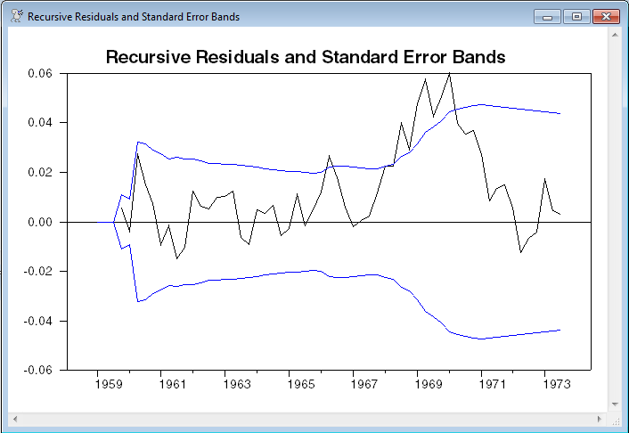
Next is a graph of the recursive residuals with the (recursively estimated) standard error bands. This doesn’t form a formal test; however, if there is a break, it’s likely that the residuals will, for a time, lie outside the bands until the coefficients or variance estimates adjust. (Graph).

set lower = -2*sighist

set upper = 2*sighist

graph(header="Recursive Residuals and Standard Error Bands") 3

# rresids

# lower / 2

# upper / 2

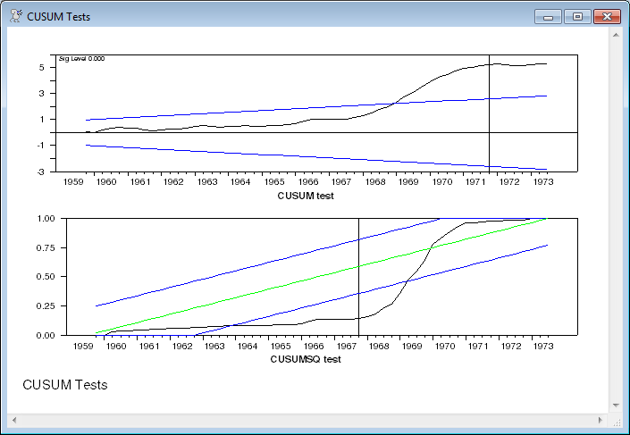
Next is the more formal CUSUM test (Brown, Durbin and Evans, 1975). Under the null, the cumulated sums of the recursive residuals should act like a random walk. If there is a structural break, they will tend to drift above the bounding lines, which here are set for the .05 level. (Graph).

set cusum = cusum/sqrt(%seesq)

set upper5 rstart 1973:3 = .948*sqrt(%ndf)*$

(1+2.0*(t-rstart+1)/%ndf)

set lower5 rstart 1973:3 = -upper5

graph(header="CUSUM test") 3

# cusum

# lower5 / 2

# upper5 / 2

This can be done more simply with the @CUSUMTESTS procedure, which does both the CUSUM test and the CUSUMQ test (for the square). The CUSUMQ test is mainly aimed at testing stability of the variance. @CUSUMTESTS takes the recursive residuals as the input series: (Graph)

@cusumtests rresids

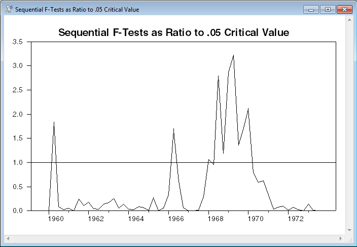
The final graph is a set of one-step Chow predictive F-tests. This is basically the same information as the recursive residuals graph with a different presentation. Again, this is an informal test. This graph is designed to present not the sequential F’s themselves, but the F’s scaled by the .05 critical value. At the start of the sample, the F’s are based upon very few denominator degrees of freedom, so F’s that are quite large may very well be insignificant. Anything above the “1” line (shown on the graph with the help of the VGRID option) is, individually, statistically significant at the .05 level. Consistent with the above, there is an indication of some form of break around 1968-1970.

set seqf = (t-rstart)*(cusumsq-cusumsq{1})/cusumsq{1}

set seqfcval rstart+1 * = seqf/%invftest(.05,1,t-rstart)

graph(vgrid=||1.0||,header=$

"Sequential F-Tests as Ratio to .05 Critical Value")

# seqfcval

Full Program

open data auto1.asc
cal(q) 1959:1
data(format=prn,org=columns) 1959:1 1973:3 x2 x3 y
*
* The StabTest procedure does the Hansen test for parameter instability
*
@stabtest y 1959:1 1973:3
# constant x2 x3
*
* Chow predictive test over the next two years after 1971:3
*
linreg(noprint) y 1959:1 1971:3
# constant x2 x3
compute rss1=%rss,ndf1=%ndf
linreg(noprint) y 1959:1 1973:3
# constant x2 x3
compute f=((%rss-rss1)/8)/(rss1/ndf1)
cdf(title="Chow Predictive Test") ftest f 8 ndf1
*
* Tests and graphs based upon recursive estimation
*
rls(sehist=sehist,cohist=cohist,sighist=sighist,$
csum=cusum,csquared=cusumsq) y 1959:1 1973:3 rresids
# constant x2 x3
*
* rstart is the first observation without a perfect fit
*
compute rstart=%regstart()+%nreg
*
* This graphs the recursive residuals with the upper and lower two
* (recursively generated) standard error bands.
*
set lower = -2*sighist
set upper = 2*sighist
graph(header="Recursive Residuals and Standard Error Bands") 3
# rresids
# lower / 2
# upper / 2
*
* CUSUM test with upper and lower bounds (done directly)
*
set cusum = cusum/sqrt(%seesq)
set upper5 rstart 1973:3 = .948*sqrt(%ndf)*$
(1+2.0*(t-rstart+1)/%ndf)
set lower5 rstart 1973:3 = -upper5
graph(header="CUSUM test") 3
# cusum
# lower5 / 2
# upper5 / 2
*
* Same thing done with @CUSUMTESTS
*
@cusumtests rresids
*
* Sequential F-Tests. These are generated quite easily using the
* cumulated sum of squares from RLS.
*
set seqf = (t-rstart)*(cusumsq-cusumsq{1})/cusumsq{1}
set seqfcval rstart+1 * = seqf/%invftest(.05,1,t-rstart)
graph(vgrid=||1.0||,header=$
"Sequential F-Tests as Ratio to .05 Critical Value")
# seqfcval

Output

Linear Regression - Estimation by Least Squares

Dependent Variable Y

Quarterly Data From 1959:01 To 1973:03

Usable Observations 59

Degrees of Freedom 56

Centered R^2 0.9752051

R-Bar^2 0.9743196

Uncentered R^2 0.9999927

Mean of Dependent Variable -7.840375448

Std Error of Dependent Variable 0.136144777

Standard Error of Estimate 0.021817336

Sum of Squared Residuals 0.0266557854

Regression F(2,56) 1101.2667

Significance Level of F 0.0000000

Log Likelihood 143.5001

Durbin-Watson Statistic 0.3491

Variable Coeff Std Error T-Stat Signif

************************************************************************************

1. Constant -1.042931912 0.296167628 -3.52142 0.00086159

2. X2 -0.672643745 0.101443769 -6.63071 0.00000001

3. X3 0.850876953 0.051136410 16.63936 0.00000000

Hansen Stability Test

Test Statistic P-Value

Joint 3.18257640 0.00

Variance 0.42303692 0.06

Constant 0.80811736 0.01

X2 0.80476019 0.01

X3 0.80124230 0.01

Chow Predictive Test

F(8,48)= 0.18421 with Significance Level 0.99201471

Linear Regression - Estimation by Recursive Least Squares

Dependent Variable Y

Quarterly Data From 1959:01 To 1973:03

Usable Observations 59

Degrees of Freedom 56

Centered R^2 0.9998482

R-Bar^2 0.9998428

Uncentered R^2 0.9999922

Mean of Dependent Variable -7.432812953

Std Error of Dependent Variable 1.739982439

Standard Error of Estimate 0.021817336

Sum of Squared Residuals 0.0266557848

Log Likelihood 143.5001

Durbin-Watson Statistic 0.2750

Variable Coeff Std Error T-Stat Signif

************************************************************************************

1. Constant -1.042931929 0.296167625 -3.52142 0.00086159

2. X2 -0.672643724 0.101443768 -6.63071 0.00000001

3. X3 0.850876972 0.051136409 16.63936 0.00000000

Graphs