GARCHVIRFDIAG.RPF

GARCHIRFDIAG.RPF is an example of computing the Volatility Impulse Response (VIRF) for a GARCH model which doesn't have a "VECH" form. It can be applied to models estimated with restricted correlations (CC or DCC), with VARIANCES=SIMPLE (default), SPILLOVER or VARMA. It does not work with VARIANCES=EXPONENTIAL or KOUTMOS as those don't have closed-form variance extrapolations.

After estimating a GARCH model of the appropriate form, such as the CC with spillover done here:

garch(p=1,q=1,mv=cc,variances=spillover,hmatrices=hh,rvectors=rv) / xjpn xfra xsui

use the @MVGARCHVarMats procedure (with the repeat of the VARIANCES option) to compute the matrices which govern the variance recursion:

@MVGARCHVarMats(variances=spillover)

This creates \(N \times N\) matrices %%VAR_A and %%VAR_B which govern the evolution of the variances (not the entire covariance matrix, which is possible with a VECH form for the GARCH model).

Unlike the impulse response in a linear model like a VAR, the volatility impulse response isn't linear in the shock size. Instead it makes sense to look at a historical episode and see what the effect is of the residuals at that time period. Here, this is done using entry 1241:

compute t0=1241

compute eps0=rv(t0).^2

compute sigma0=%xdiag(hh(t0))

compute shock=eps0-sigma0

The "shock" is the difference between the squared residuals and the GARCH-estimated variance at the time.

The following does the calculation of a 100 period response of the variances of the three processes. At step 1, the only addition is from the shock itself which uses just the "A" matrix. After that, both the "A" and "B" matrices apply to the previous period's variance response. (This is the difference in forecasts of the variance due to the addition of the shock).

compute nstep=100

dec vect[series] virf1241(%nvar)

do i=1,%nvar

set virf1241(i) 1 nstep = 0.0

end do i

do step=1,nstep

if step==1

compute hvec=%%var_a*shock

else

compute hvec=(%%var_a+%%var_b)*hvec

compute %pt(virf1241,step,hvec)

end do step

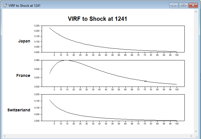
The VIRF's are then graphed (see results below)

Full Program

open data g10xrate.xls
data(format=xls,org=columns) 1 6237 usxjpn usxfra usxsui
*
set xjpn = 100.0*log(usxjpn/usxjpn{1})
set xfra = 100.0*log(usxfra/usxfra{1})
set xsui = 100.0*log(usxsui/usxsui{1})
*
dec vect[strings] glabels(3)
compute glabels=||"Japan","France","Switzerland"||
*
* This can be applied to models estimated with restricted correlations
* (CC or DCC), with VARIANCES=SIMPLE (default), SPILLOVER or VARMA. It
* does not work with VARIANCES=EXPONENTIAL or KOUTMOS as those don't
* have closed-form variance extrapolations.
*
garch(p=1,q=1,mv=cc,variances=spillover,pmethod=simplex,piters=20,hmatrices=hh,rvectors=rv) / xjpn xfra xsui
*
* This pulls the matrices for a variance recursion out of the output
* from the GARCH model. Do this immediately after the GARCH instruction
* and repeat the VARIANCES option.
*
@MVGARCHVarMats(variances=spillover)
*
* Compute VIRF at t=1241
*
compute t0=1241
compute eps0=rv(t0).^2
compute sigma0=%xdiag(hh(t0))
*
compute shock=eps0-sigma0
*
compute nstep=100
*
dec vect[series] virf1241(%nvar)
do i=1,%nvar
   set virf1241(i) 1 nstep = 0.0
end do i
*
do step=1,nstep
   if step==1
      compute hvec=%%var_a*shock
   else
      compute hvec=(%%var_a+%%var_b)*hvec
   compute %pt(virf1241,step,hvec)
end do step
*
spgraph(vfields=%nvar,ylabels=glabels,header="VIRF to Shock at 1241")
do i=1,%nvar
    graph(min=0.0,column=1,row=i,picture="*.###",vticks=5)
    # virf1241(i) 1 nstep
end do i
spgraph(done)

Graph

Japan and Switzerland show the typical pattern of a responses to a shock which is historically large relative to its variance. The France response is positive (so it's also above its variance at the episode studied) but is probably not as extreme as the other two series, so the feedback from the other countries pushes the France variance higher in the early part.