GCONTOUR.RPF

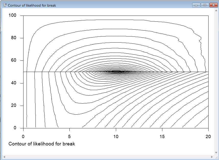
GCONTOUR.RPF is an example of a contour graph.

This creates a series which is mean 0 through entry 50, and mean 10 from 51 through the end of the sample. We use a SEED to ensure that the graph can be reproduced.

seed 95035

set x 1 100 = %if(t>50,10,0)+%ran(1.0)

The goal is to generate a graph of the contours of the log likelihood for a model with a break from a zero mean process to an unknown non-zero mean process at an unknown break point. This generates grids for the break location (each entry number from 1 to 100) and for the post-break mean values, which we limit to the range from 0.2 to 20.0 by steps of .2:

compute breaks=%seqa(1.0,1.0,100)

compute mus =%seqa( .2, .2,100)

This generates the log likelihood for all the combinations of mus and breaks. The sum of squares for a break after entry \(B\) to a new mean of \(\mu\) is

\(\sum\limits_t^{} {x_t^2 } - 2\mu \sum\limits_{t > B} {x_t } + (T - B)\mu ^2\)

What is computed is the concentrated log likelihood, assuming Normal residuals, and fixed, but unknown, variance. To compute the sums of squares for different choices for \(B\), we need the first two sums (the second of which is a whole series of partial sums). This generates as the series OVER the sum of X for elements above entry number T.

acc x / ax
set over = ax(100)-ax(t)

and this is the sum of squares of X

compute x2=%normsqr(x)

Finally, this fills in the grid of values, with mu varying across rows and the breakpoint across columns:

dec rect f(100,100)

ewise f(i,j)=-50.0*log((x2-2*mus(i)*over(fix(breaks(j)))+(100-breaks(j))*mus(i)^2)/100.0)

This does the contour graph with a grid line across the actual break (50). The X axis values are the MUS and the Y axis values are the BREAKS.

gcontour(x=mus,y=breaks,f=f,vgrid=||50||)

Full Program

seed 95035

set x 1 100 = %if(t>50,10,0)+%ran(1.0)

* The sum of squared residuals for a break between B and B+1 and a

* post-break mean of mu (pre-break mean assumed to be zero) is

* sum (all t) of x^2 - 2*mu*sum (t>B) of x + (T-B)*mu^2

* This generates a contour plot of the concentrated log likelihood,

* assuming Normal residuals, and fixed, but unknown, variance.

* Set up the grids for breaks (1,...,100) and mus (.2,.4,...,20)

compute breaks=%seqa(1.0,1.0,100)

compute mus =%seqa( .2, .2,100)

* This generates as "over" the sum of x for elements above t.

acc x / ax

set over = ax(100)-ax(t)

* Compute the sum of squares

compute x2=%normsqr(x)

* Generate the log likelihood for all the combinations of mus and breaks.

dec rect f(100,100)

ewise f(i,j)=-50.0*log((x2-2*mus(i)*over(fix(breaks(j)))+(100-breaks(j))*mus(i)^2)/100.0)

* Do the contour graph with a grid line across the actual break (50)

gcontour(footer="Contour of likelihood for break",x=mus,y=breaks,f=f,vgrid=||50||)

Graph