HAMILTON.RPF

HAMILTON.RPF uses the @MSVARSETUP procedures to estimate Hamilton’s switching model for GDP growth (Hamilton, 1994, Chapter 22). Despite the fact that it’s just one variable (not a VAR), @MSVARSETUP is used because the mean-only switch is included in it. (The mean switch makes little sense except in a self-contained model like a VAR or AR, and so isn’t included in the general single-equation @MSRegression).

The intent of the model is that the "regime" is either high growth or low growth represented by its mean value. Current (quarterly) GDP growth is modeled as the current regime-specific mean plus a four lag autoregression on the deviations of GDP growth from the lagged regime-specific mean. This means that there is a separate branch of the likelihood for each combination of current and four lags of the regime (thus 32 in all). This sets up the Markov Switching "VAR" for the one variable (G), with only means switching (SWITCH=M). (Regimes are 2 by default):

@msvarsetup(lags=4,switch=m)

# g

Because everything is recursively defined, Markov switching models need a “hard” start and end for their range, which this sets. (You lose five data points from the original data: one for creating GDP growth from GDP and four others from the 4 lags in the model).

compute gstart=1952:2, gend=1984:4

The MSVARF is the log likelihood formula, using the function brought in when you execute @MSVARSETUP:

frml msvarf = log(%MSVARProb(t))

Note that almost all of the rather complicated calculation of likelihoods is done by the procedures and functions pulled in with @MSVARSETUP.

The model is parameterized using the P matrix for the probabilities. MU has the regime-specific means. It’s a VECTOR[VECTOR], with the primary selector picking the regime, while the secondary picks the “variable” (which is just 1). So MU(1)(1) is the mean in regime 1 and MU(2)(1) is the mean in regime 2. PHI is what is used when the lag coefficients aren’t regime-dependent. It’s a VECT[RECT] where the VECTOR is over the lags and RECT over the variables. Again, with just a single variable, the latter has just (1,1) subscripts. So PHI(1)(1,1) is the first lag coefficient, PHI(4)(1,1) the last. SIGMA (again, fixed across regimes) is a $1 \times 1$ SYMMETRIC matrix.

nonlin(parmset=msparms) p

nonlin(parmset=varparms) mu phi sigma

This does the guess values by estimating the base VAR, and copying out the lag coefficients and variance from that, and giving separated values to the means (lower for regime 1, higher for regime 2). This generally works for the Hamilton model with just the switching mean. If the entire coefficient vector is switching, it may not work as well, since it is really designed with the assumption that it’s means that differ.

@msvarinitial gstart gend

This does the estimation. This uses a REJECT option to avoid doing a function evaluation if the transition matrix has any values out of range, which is possible if we are estimating the P form.

maximize(parmset=varparms+msparms,$

start=(pstar=%MSVARInit()),$

reject=%MSVARInitTransition()==0.0,$

pmethod=simplex,piters=5,method=bfgs,iters=300) $

msvarf gstart gend

The START option is evaluated at the start of each function evaluation to set the initial probabilities into the PSTAR VECTOR. Note that PSTAR has dimension 32 since it needs to cover all 32 possible combinations of regimes.

This computes the smoothed estimates of the states, and puts into PCONTRACT the probability of the lower mean regime (the first, if our guess values held up).

@msvarsmoothed gstart gend psmooth

set pcontract gstart gend = psmooth(t)(1)

To create the shading marking the recessions, create a dummy series which is 1 when the RECESSQ series is 1, and 0 otherwise. RECESSQ is 1 for NBER recessions and -1 for expansions—it’s included on the data set, but more generally can be created (for the U.S.) using the @NBERCYCLES procedure.

set contract = recessq==1

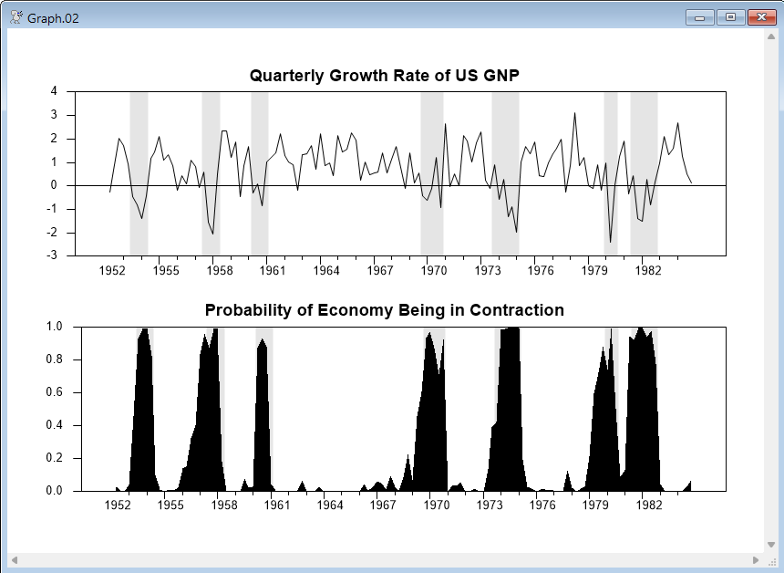
Graph the data on the top and the probability of contraction (with the recession shading) on the bottom.

spgraph(vfields=2)

graph(header="Quarterly Growth Rate of US GNP",shade=contract)

# g %regstart() %regend()

graph(style=polygon,shade=contract,$

header="Probability of Economy Being in Contraction")

# pcontract %regstart() %regend()

spgraph(done)

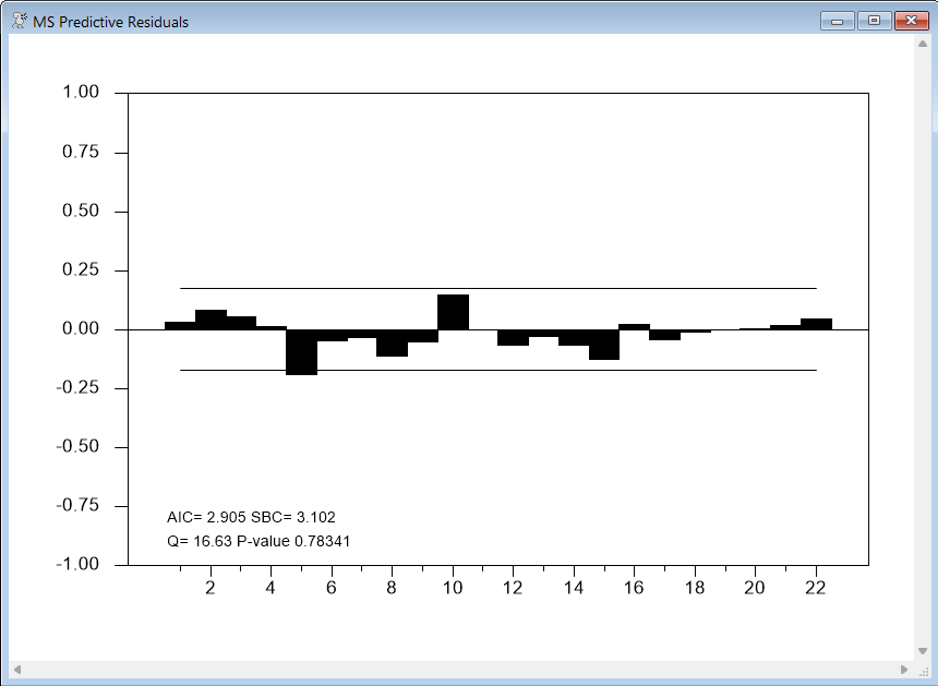
Compute the predictive probability-weighted standardized residuals and check for serial correlation.

@MSVARStdResiduals %regstart() %regend() stdu

@regcorrs(title="MS Predictive Residuals",qstat) stdu(1)

Predictive probability-weighted standardized residuals is quite a long description, but they are the proper choice for doing any diagnostics. The regime-specific residuals (the model residuals across time for a specific regime) won’t work because the model says nothing about their behavior in the time periods which aren’t part of that regime. The residuals have to be computed using the model’s predictions, weighted by the predictive probabilities for them to be serially uncorrelated. They are standardized because if the variance is switching (it isn't in this example), the regimes would be predicting different variances, so the residuals have to be standardized before being probability-weighted. If the model is correct the residuals would be expected to be serially uncorrelated. They would not, however, be expected to be Normal.

Note that, while this model fits remarkably well to this data set, attempts to fit the same basic model it to a range of data through 2000 doesn't work as well. There is only one rather modest recession between 1982 and 2000, which isn't really compatible with this estimated model.

Full Program

cal(q) 1951:1
open data gnpdata.prn
data(format=prn,org=columns) 1951:1 1984:4
*
set g = 100*log(gnp/gnp{1})
graph(header="GNP growth")
# g
*
* Set up a mean-switching model with just the one variable and four lags.
*
@msvarsetup(lags=4,switch=m)
# g
compute gstart=1952:2,gend=1984:4
frml msvarf = log(%MSVARProb(t))
*
nonlin(parmset=msparms) p
nonlin(parmset=varparms) mu phi sigma
@msvarinitial gstart gend
*
* Estimate the model by maximum likelihood.
*
maximize(parmset=varparms+msparms,$
start=(pstar=%MSVARInit()),$
reject=%MSVARInitTransition()==0.0,$
pmethod=simplex,piters=5,method=bfgs,iters=300) $
msvarf gstart gend
*
* Compute smoothed estimates of the regimes.
*
@msvarsmoothed gstart gend psmooth
set pcontract gstart gend = psmooth(t)(1)
*
* To create the shading marking the recessions, create a dummy series
* which is 1 when the recessq series is 1, and 0 otherwise. (recessq is
* 1 for NBER recessions and -1 for expansions).
*
set contract = recessq==1
*
* Graph the data on the top and the probability of contraction (with the
* recession shading) on the bottom.
*
spgraph(vfields=2)
graph(header="Quarterly Growth Rate of US GNP",shade=contract)
# g %regstart() %regend()
graph(style=polygon,shade=contract,$
header="Probability of Economy Being in Contraction")
# pcontract %regstart() %regend()
spgraph(done)
*
* Compute predictive probability-weighted standardized residuals and
* check for serial correlation.
*
@MSVARStdResiduals %regstart() %regend() stdu
@regcorrs(title="MS Predictive Residuals",qstat) stdu(1)

Output

MAXIMIZE - Estimation by BFGS

Convergence in 16 Iterations. Final criterion was 0.0000076 <= 0.0000100

Quarterly Data From 1952:02 To 1984:04

Usable Observations 131

Function Value -181.2634

Variable Coeff Std Error T-Stat Signif

************************************************************************************

1. MU(1)(1) -0.358820781 0.269293336 -1.33245 0.18271129

2. MU(2)(1) 1.163515539 0.074938767 15.52622 0.00000000

3. PHI(1)(1,1) 0.013483699 0.122703202 0.10989 0.91249762

4. PHI(2)(1,1) -0.057524408 0.140939795 -0.40815 0.68316443

5. PHI(3)(1,1) -0.246986125 0.113688556 -2.17248 0.02981947

6. PHI(4)(1,1) -0.212923197 0.111088287 -1.91670 0.05527574

7. SIGMA(1,1) 0.591366233 0.104445738 5.66195 0.00000001

8. P(1,1) 0.754669349 0.096789430 7.79702 0.00000000

9. P(1,2) 0.095914539 0.040334418 2.37798 0.01740765

Graphs