MONTESVAR.RPF

MONTESVAR.RPF is an example of Monte Carlo (importance sampling) integration for impulse responses in a structural VAR. An alternative which does Random Walk Metropolis-Hastings rather than importance sampling is provided in MONTESVAR_MH.RPF.

Full Program

open data haversample.rat
calendar(q) 1959
data(format=rats) 1959:1 2006:4 ffed fm1 fnh gdph lr dgdp
*
compute lags=4
compute nvar=6
compute nstep=16
compute ndraws=10000
*
set ffed = ffed*.01
set lr   = lr*.01
log gdph
log dgdp
log fnh
log fm1
*
* In this section, we set up a system for a structural model. First,
* estimate the VAR by OLS.
*
system(model=varmodel)
variables ffed fm1 gdph dgdp lr fnh
lags 1 to lags
det constant
end(system)
*
estimate(cvout=vmat)
compute xxx=%xx
*
* Save a factor of the inv(X'X) matrix from the VAR, and the OLS
* coefficients.
*
compute fxx    =%decomp(xxx)
compute betaols=%modelgetcoeffs(varmodel)
compute ncoef =%rows(fxx)
*
* Create the set of non-linear parameters, and the "A" formula for
* CVMODEL. Since these are all off-diagonal coefficients, all zeros
* has a good chance of working as guess values.
*
nonlin(parmset=simszha,zeros) a12 a21 a23 a24 a31 a36 $
   a41 a43 a46 a51 a53 a54 a56
compute nfree=13
*
dec frml[rect] afrml
frml afrml = ||1.0   ,a12 ,0.0   ,0.0   ,0.0 ,0.0|$
               a21   ,1.0 ,a23   ,a24   ,0.0 ,0.0|$
               a31   ,0.0 ,1.0   ,0.0   ,0.0 ,a36|$
               a41   ,0.0 ,a43   ,1.0   ,0.0 ,a46|$
               a51   ,0.0 ,a53   ,a54   ,1.0 ,a56|$
               0.0   ,0.0 ,0.0   ,0.0   ,0.0 ,1.0||
*
declare rect fsigmad betaols betadraw
declare symm sigmad
*
* Compute the maximum of the log of the marginal posterior density for
* the A coefficients with a prior of the form |D|**(-delta). Delta
* should be at least (nvar+1)/2.0 to ensure an integrable posterior
* distribution.
*
compute delta=3.5
cvmodel(parmset=simszha,dfc=ncoef,pdf=delta,dmatrix=marginalized,method=bfgs) vmat afrml
dec rect faxx
*
* axbase is the maximizing vector of coefficients.
*
compute [vector] axbase=%parmspeek(simszha)
*
* <<faxx>> is a factor of the (estimated) inverse Hessian at the final
* estimates. This gets scaled slightly to fatten up the tails a bit.
*
compute faxx=1.2*%decomp(%xx)
*
* <<scladjust>> is used to prevent overflows when computing the weight
* function.
*
compute scladjust=%funcval
*
* <<nu>> is the degrees of freedom for the multivariate Student used in
* drawing A's.
*
compute nu=30.0
*
* We need to save the draws in %%RESPONSES as described in the manual
* (for use with MCGRAPHIRF). We also need a series to hold the weights.
*
set weights 1 ndraws = 0.0
declare vect au(%nreg)
declare vect dbase d(nvar)
*
* This is the standard name used by the MCGraphIRF procedure
*
declare vect[rect] %%responses(ndraws)
*
* sumwt and sumwt2 will hold the sum of the weights and the sum of
* squared weights.
*
compute sumwt=0.0
compute sumwt2=0.0
infobox(action=define,progress,lower=1,upper=ndraws) "Monte Carlo Integration"
*
* Antithetic acceleration is used for the lag coefficients only, so on
* odd number draws, we generate a new sigma matrix, and a set of changes
* to the lag coefficients, then on the even ones, we generate a new draw
* with the sign switched on the deltas to the lag coefficients.
*
do draw=1,ndraws
   if %clock(draw,2)==1 {
      *
      * Do a draw for the coefficients from a multivariate t density and
      * "poke" it back into the parmset so the AFRML can get the new
      * values. Save the log kernel of the draw into <<idensity>>.
      *
      compute au      =%rant(nu)
      compute idensity=%ranlogkernel()
      compute %parmspoke(simszha,axbase+faxx*au)
      *
      * Evaluate the model at the draw for the coefficients. Save the
      * log likelihood.
      *
      cvmodel(parmset=simszha,dfc=ncoef,pdf=delta,dmatrix=marginalized,dvector=ddiag,method=evaluate) vmat afrml
      compute pdensity=%funcval
      *
      * Compute the weight value by exp'ing the difference between the
      * two densities, with a scale adjustment term to prevent overflow.
      *
      compute weight =exp(pdensity-scladjust-idensity)
      *
      * Conditioned on A, make a draw for the D matrix
      *
      ewise d(i)      =(%nobs/2.0)*ddiag(i)/%rangamma(.5*(%nobs-ncoef)+delta+1)
      *
      * Combine D and A to generate the draw for a factor of sigma.
      *
      compute a       =afrml(1)
      compute fsigmad =inv(a)*%diag(%sqrt(d))
      *
      * Compute the + draw for coefficients
      *
      compute betau   =%ranmvkron(fsigmad,fxx)
      compute betadraw=betaols+betau
   }
   else {
      *
      * Compute the - draw for the coefficients
      *
      compute betadraw=betaols-betau
   }

   compute %modelsetcoeffs(varmodel,betadraw)
   compute nshock=3
   *
   * Extract the P, U and I shocks
   *
   compute shockpui=%xcol(fsigmad,3)~%xcol(fsigmad,5)~%xcol(fsigmad,6)
   impulse(noprint,model=varmodel,factor=shockpui,$
      flatten=%%responses(draw),steps=nstep) nvar
   *
   * Save the draw weights
   *
   compute sumwt   =sumwt+weight
   compute sumwt2 =sumwt2+weight^2
   compute weights(draw)=weight
   infobox(current=draw)
end do draw
infobox(action=remove)
*
* The efficacy of importance sampling depends upon function being
* estimated, but the following is a simple estimate of the number of
* effective draws.
*
disp "Effective sample size" sumwt^2/sumwt2
*
* Normalize the weights to sum to 1.0
*
set weights 1 ndraws = weights/sumwt
*
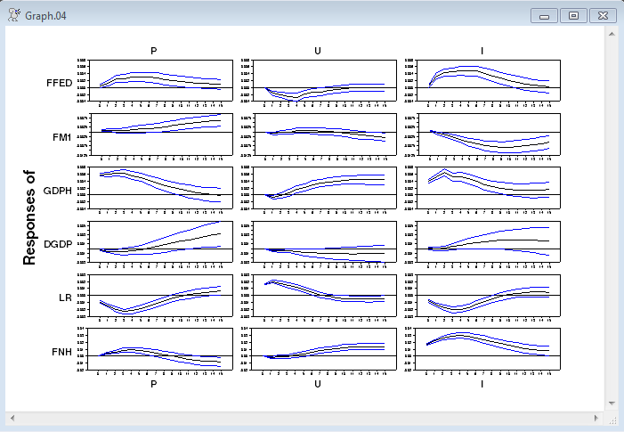
@MCGraphIRF(model=varmodel,center=mean,page=all,weights=weights,$
shocklabels=||"P","U","I"||)

Output

The effective sample size depends upon random numbers and so the results will not be exactly reproducible.

(VAR lag coefficient output)

Covariance Model-Marginal Posterior - Estimation by BFGS

Convergence in 32 Iterations. Final criterion was 0.0000043 <= 0.0000100

Observations 188

Function Value 3867.5518

Prior DF 3.5000

Variable Coeff Std Error T-Stat Signif

************************************************************************************

1. A12 -0.210169018 0.328503264 -0.63978 0.52231722

2. A21 0.239494036 0.266017748 0.90029 0.36796411

3. A23 -0.130823823 0.104316657 -1.25410 0.20980460

4. A24 -0.376127996 0.222527257 -1.69026 0.09097902

5. A31 -0.007454838 0.068674529 -0.10855 0.91355690

6. A36 -0.232790224 0.028240889 -8.24302 0.00000000

7. A41 -0.046540455 0.030370724 -1.53241 0.12542085

8. A43 0.057057884 0.034831917 1.63809 0.10140251

9. A46 -0.014429582 0.015065034 -0.95782 0.33815382

10. A51 0.098851055 0.017241422 5.73335 0.00000001

11. A53 0.156988068 0.021989863 7.13911 0.00000000

12. A54 0.035038164 0.049088412 0.71378 0.47536528

13. A56 0.007954866 0.009414004 0.84500 0.39810888

Effective sample size 500.61268

Graph