MONTESUR.RPF

MONTESUR.RPF uses Gibbs sampling to analyze the impulse response functions for a near-VAR (a VAR with some lagged variables excluded from some of the equations).

Because the model isn't symmetric in the variables, the likelihood can't be decomposed in the simple fashion that is available for "OLS" VAR's and used in (for instance) the procedure @MONTEVAR. For those, the covariance matrix of residuals $\Sigma$ has an unconditional distribution and so can be drawn directly and then the lag coefficients ($\bf{Β}$) can be drawn conditionally on $\Sigma$. With the asymmetrical VAR, the density of $\Sigma$ depends upon $\bf{Β}$, hence the use of the use of the Gibbs sampler to alternate between drawing $\Sigma$ and $\bf{Β}$ given $\Sigma$. This uses the @SURGibbsSetup procedures to handle the specialized calculations.

Each Gibbs sweep requires doing (in effect) a full estimate of the near-VAR by Seemingly Unrelated Regressions—for a large VAR, this can become computationally burdensome. There are more efficient sampling algorithms which can be used for models with specific structures—see the Cushman and Zha(1997) replication for an example.

This uses a Cholesky factorization to identify the shocks. A structural contemporaneous model (a "near-SVAR") is quite a bit more difficult. An example of that is provided as MONTENEARSVAR.RPF.

A near-VAR or any other type of multiple equation linear model with non-matching explanatory variables has to be done using the techniques described for general priors in multivariate systems. The difference between a technically correct analysis of a near-VAR system and a VAR with a prior is quite minor—the block exclusion in the near-VAR is really just an (infinitely) tight prior on some of the coefficients.

This requires inverting the precision matrix for the entire system. This could be extremely time-consuming for a large model—with the time required for inversion going up with the cube of the size, a 1200 coefficient model will take (roughly) 64 times as long as a 300 coefficient model.

Although the procedure for drawing from a near-VAR is equivalent to estimating a SUR model each time you get a new covariance matrix, the SUR instruction, in addition to having to invert the big matrix, also has to compute the cross product matrix of the data. Since the data information is the same from sweep to sweep, we can eliminate that time cost by organizing the data information in advance. That can be done with the @SURGIBBSSETUP procedure group which handles the interactions between the drawing procedure and the data. If you are interested in the technical details, they are covered as part of the Bayesian Econometrics e-course.

The MONTESUR.RPF example does a two variable near-VAR, where one variable is excluded from the other’s equation. However, the same basic program can be adapted to create draws for any other (linear) SUR model. The draws are used to compute impulse response functions, which are saved and later graphed as described in the section on regular VAR's. The following sets up the model by defining the two equations and GROUPing them into a model. See "xxx"for different ways to handling this step that might be more appropriate for larger systems.

equation gdpeq loggdp

# loggdp{1 to lags} logm1{1 to lags} constant

equation m1eq logm1

# logm1{1 to lags} constant

* Create the model

group surmodel m1eq gdpeq

The call to @SURGibbsSetup takes the model and sets up all the information required for interacting with the data. It figures out what series and lags are needed and computes the cross product matrix of them and organizes information for later use.

@SURGibbsSetup surmodel

This uses SUR to initialize the sampler—as we have the sampler set up, all that’s needed for that are the coefficients (into BDRAW).

sur(model=surmodel)

compute ntotal=%nreg

compute bdraw=%beta

compute wishdof=%nobs

Inside the draw loop, the first step is to compute the covariance matrix of residuals at the current beta. This uses one of the other procedures that is pulled in by @SURGIBBSSETUP to compute T times the covariance matrix at the current set of coefficients.

compute covmat=SURGibbsSigma(bdraw)

This next does a draw for the precision matrix (inverse of the covariance matrix) conditional on the current coefficients (through COVMAT).

compute hdraw=%ranwishartf(%decomp(inv(covmat)),wishdof)

Compute the information obtained by interacting the precision matrix and the data. These are precision matrix for the coefficients (HDATA) and precision matrix times the mean (HBDATA). If you had an actual prior (besides the zero restrictions), you would adjust HDATA and HBDATA to take those into account before continuing.

@SURGibbsDataInfo hdraw hdata hbdata

This is the “hot spot” of the calculation, as this requires (internally) inverting the (potentially very) large precision matrix HDATA.

compute bdraw=%ranmvposthb(hdata,hbdata)

The following is the “bookkeeping” section, which is executed once we’re past the burn-in. The calculations above have all used only the precision matrix for the residuals, so we have to invert that now to get the covariance matrix (into SIGMAD). This does Cholesky factor shocks. As with the full VAR, you can use any other “FACTOR” matrix here to deal with just-identified or non-orthogonalized shocks. However, the (relatively) simple Gibbs sampler can’t be used with an overidentified structural model.

compute %modelsetcoeffs(surmodel,bdraw)

compute sigmad=inv(hdraw)

impulse(noprint,model=surmodel,factor=%decomp(sigmad),$

steps=nsteps,flatten=%%responses(draw))

Full Program

compute lags=4 ;*Number of lags

compute nsteps=16 ;*Number of response steps

compute nburn =5000 ;*Burn-in draws

compute ndraws=25000 ;*Keeper draws

open data haversample.rat

calendar(q) 1959

data(format=rats) 1959:1 2006:4 fm1 gdph

set loggdp = 100.0*log(gdph)

set logm1 = 100.0*log(fm1)

equation gdpeq loggdp

# loggdp{1 to lags} logm1{1 to lags} constant

equation m1eq logm1

# logm1{1 to lags} constant

* Create the model

group surmodel m1eq gdpeq

compute nvar=%modelsize(surmodel)

* Do set up for Gibbs sampling on SUR model

@SURGibbsSetup surmodel

**********************************************

* Do a SUR to get a set of estimates to initialize the Gibbs sampler.

sur(model=surmodel)

compute ntotal=%nreg

compute bdraw=%beta

compute wishdof=%nobs

* For saving the IRF's

declare vect[rect] %%responses(ndraws)

infobox(action=define,progress,lower=-nburn,upper=ndraws) $

"Gibbs Sampling"

do draw=-nburn,ndraws

* Compute covariance matrix of residuals at the current beta

compute covmat=SURGibbsSigma(bdraw)

* Do a draw for the precision matrix conditional on beta

compute hdraw=%ranwishartf(%decomp(inv(covmat)),wishdof)

* Compute the required information with the interaction between

* the precision matrix and the data

@SURGibbsDataInfo hdraw hdata hbdata

* Draw coefficients given the precision matrix hdraw

compute bdraw=%ranmvposthb(hdata,hbdata)

infobox(current=draw)

if draw<=0

* Do the bookkeeping here.

compute %modelsetcoeffs(surmodel,bdraw)

compute sigmad=inv(hdraw)

impulse(noprint,model=surmodel,factor=%decomp(sigmad),$

steps=nsteps,flatten=%%responses(draw))

end do draw

infobox(action=remove)

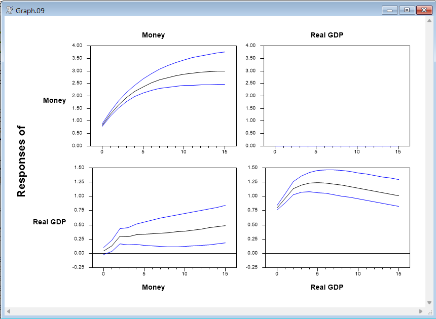
@MCGraphIRF(model=surmodel,center=median,page=all,$

picture="*.##",varlabels=||"Real GDP","Money"||)

Graph

By construction, the response of Money to a real GDP shock is zero.