@ROLLREG is a procedure to do various types of "rolling" linear regressions. This was written originally by economists at the Bank of Canada.

 

@ROLLREG( options )   depvar first last

# list of explanatory variables (in Regression Format)

Parameters

Options for controlling rolling samples

MOVE=width of moving window

Starting with a regression from first to first+MOVE width-1, adds observations to the end and drops them from the start one at a time until it does a regression from last-MOVE width+1 to last, that is, there are MOVE width observations in each regression

 

ADD=end of initial period

Starting with a regression from first to the ADD option value, adds one observation at a time to the end of the range until it does a regression from first to last. What ADD does could be handled more efficiently by the RLS instruction.

 

DROP=start of last regression range

Starting with a regression from first to last, drops one observation at a time from the beginning of the range until it does a regression from DROP option value to last

Other options

ROBUST/[NOROBUST]

Uses the ROBUSTERRORS option to calculate the standard errors.

LAGS=number of lags to use with the ROBUST option [0]

LWINDOW=[NEWEY]/BARTLETT/DAMPED/PARZEN/QUADRATIC

Chooses lag window type if LAGS>0.
 

COHISTORY=(output) VECT[SERIES] for the coefficients

SEHISTORY=(output) VECT[SERIES] for the standard errors of the coefficients

SIGHISTORY=(output) SERIES for the regression standard errors

These are all similar to the options for the RLS instruction.

 

FHISTORY=(output) SERIES with regression F's

 

PRINT/[NOPRINT]

WINDOW="title for print window"

Prints a table with the coefficient estimates. With WINDOW, it goes into a separate Report Window.

 

GRAPH/[NOGRAPH]

With GRAPH, graphs the coefficients with two standard error bands.

Example

open data auto1.asc

cal(q) 1959:1

data(format=prn,org=columns) 1959:1 1973:3 x2 x3 y

*

* If you use the GRAPH option, a separate graph is generated for each

* coefficient with the running estimates and two standard error bands.

* You can wrap the use of @RollReg in an SPGRAPH to make those panes on

* a single page.

*

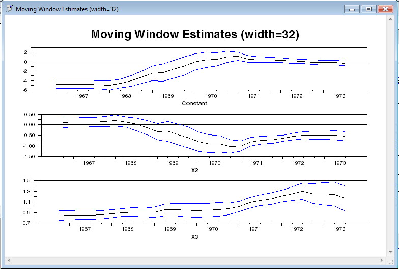
* Moving window estimates, using a window of width 32

*

spgraph(vfields=3,header="Moving Window Estimates (width=32)")

@rollreg(graph,move=32) y

# constant x2 x3

spgraph(done)

*

* Expanding window estimates with first regression running through 1965:1

*

spgraph(vfields=3,header="Expanding Window Estimates")

@rollreg(graph,add=1965:1) y

# constant x2 x3

spgraph(done)

*

* Contracting window estimates with final regression starting in 1969:1

*

spgraph(vfields=3,header="Contracting Window Estimates")

@rollreg(graph,drop=1969:1) y

# constant x2 x3

spgraph(done)

*

* Other options

*

* Displaying coefficients in a report window

*

@rollreg(print,move=32) y

# constant x2 x3

*

* Saving into a VECT[SERIES]

*

@rollreg(cohist=cohist,move=32) y

# constant x2 x3

copy(format=free,org=colums,unit=output) / cohist

*

* With HAC standard errors

*

spgraph(vfields=3,header="Moving Window Estimates with HAC Standard Errors")

@rollreg(graph,robust,lags=4,lwindow=newey,move=32) y

# constant x2 x3

spgraph(done)

Sample Output

This is how a graph looks if you wrap the procedure call inside an SPGRAPH. If you don't, there will be a separate graph for each coefficient.

 

 

 

This is what is produced by the PRINT option.

 

 ENTRY       Constant           X2              X3

 1966:04  -4.761185930838  0.113767505558  0.842047258451

 1967:01  -4.797516325896  0.127822358489  0.848764103881

 1967:02  -4.795956067159  0.127212999127  0.848474325303

 1967:03  -4.802042019714  0.128265095933  0.848171710544

 1967:04  -4.902503871897  0.161834240309  0.860841263026

 1968:01  -5.002516431152  0.200518123322  0.878949334168

 1968:02  -4.626710143013  0.137656716146  0.897886120707

 1968:03  -4.068189217665  0.026898029693  0.907400566544

 1968:04  -3.304843471982 -0.141646296819  0.902382342489

 1969:01  -2.437531479678 -0.327921595905  0.902250761965

 1969:02  -2.289279023782 -0.314337834388  0.950659775805

 1969:03  -1.597996335957 -0.460857629550  0.952798179229

 1969:04  -0.909938962533 -0.614891405392  0.946135232878

 1970:01  -0.036819078916 -0.809968863930  0.938343462725

 1970:02   0.397971797836 -0.897480533753  0.944999513773

 1970:03   0.473404681790 -0.901537022637  0.958250140200

 1970:04   1.066026825960 -1.015792311129  0.973136727987

 1971:01   1.155877707395 -0.999391768011  1.012127476841

 1971:02   0.541729178105 -0.798612203409  1.086147971455

 1971:03   0.424722362557 -0.733379136735  1.129566308289

 1971:04   0.391077588596 -0.700256785593  1.157662831523

 1972:01   0.324641947446 -0.638510443670  1.209122829016

 1972:02   0.140772446193 -0.554579418902  1.257082756085

 1972:03   0.039154529481 -0.493866185046  1.299209817436

 1972:04  -0.126632124011 -0.499396515712  1.254460127064

 1973:01  -0.160657115324 -0.496774613173  1.249389387485

 1973:02  -0.185624950645 -0.494028993024  1.246763022871

 1973:03  -0.332617872518 -0.539890833825  1.162344575656

 

Copyright © 2026 Thomas A. Doan