SIMPLERBC.RPF

SIMPLERBC.RPF is an example of solving a DSGE, producing impulse responses. It's an example from the description of the DSGE instruction and @DLMIRF procedure.

Full Program

dec real beta rho mu alpha delta
dec series r c k y theta
*
frml(identity) f1 = 1 - (beta*r{-1}*c/c{-1})
frml(identity) f2 = r - (theta*alpha*k{1}^(alpha-1)+1-delta)
frml(identity) f3 = y - (theta*k{1}^alpha)
frml(identity) f4 = y - (c + k - (1-delta)*k{1})
frml f5 = log(theta) - (rho*log(theta{1})+(1-rho)*mu)
*
group simplerbc f1 f2 f3 f4 f5
compute alpha=.3,delta=.15,rho=.9,beta=.95,mu=4.0
dsge(model=simplerbc,expand=loglin,steady=ss,a=adsge,f=fdsge) y c k r theta
*
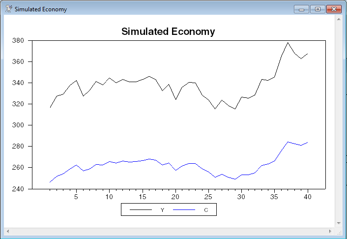
* Simulate 40 periods of the model with productivity shocks that are
* have a standard deviation of .02 (2%, since theta is in log form).
* Since this creates random draws for the log deviations from
* steady-state, we need to exp and rescale by the steady state values to
* get simulated levels.
*
dlm(a=adsge,f=fdsge,presample=ergodic,sw=.02^2,type=simulate) 1 40 xsims
set y = exp(xsims(t)(1))*ss(1)
set c = exp(xsims(t)(2))*ss(2)
graph(header="Simulated Economy",key=below) 2
# y
# c
*
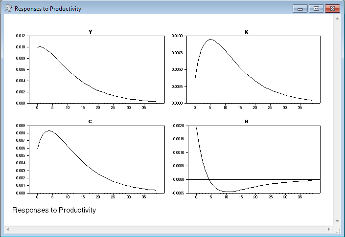
* Compute responses to size .01 productivity shock. (If you don't
* rescale the F input matrix, the shock will be 1.0 in log form, or
* 271.8%, causing a rather dramatic response to interest rates).
*
@dlmirf(a=adsge,f=fdsge*.01,steps=40,page=byshock,$
variables=||"Y","C","K","R"||,shocks=||"Productivity"||)

Graphs