SHUTDOWN.RPF

SHUTDOWN.RPF is an example of calculating a variant of impulse response in a VAR which shuts down the dynamic response of a variable. This is based upon Bachmann and Sims(2012) with a reconstructed and extended data set.

The raw data are US data originally taken from FRED. GCECI is real government consumption and investment, GDPC1 is real GDP, UMCSENT is consumer sentiment and CNP16OV is non-institutional population age 16 and over. These are read in from a RATS format file and renamed with more descriptive titles:

cal(q) 1960:1

open data shutdowndata.rat

data(format=rats) / REALGOVT<<'GCEC1' REALGDP<<'GDPC1' CONF<<'UMCSENT' POP<<'CNP16OV'

The three variables used in the VAR are log government spending, log GDP and (log) consumer confidence, for which the consumer sentiment is used. Spending and GDP are transformed to per capita numbers.

set lg_pc = 100.0*log(realgovt/pop)

set yg_pc = 100.0*log(realgdp/pop)

set lconf = 100.0*log(conf)

A four lag VAR is estimated, with the variables in the order G (government spending), C (confidence) and Y (output). G is put first on the assumption that G cannot respond within the quarter.

system(model=gcy)

variables lg_pc lconf yg_pc

lags 1 to 4

det constant

end(system)

estimate

The goal is to find a sequence of own shocks to the confidence variable which will zero out all effects of a (Cholesky) impact shock to government spending over the horizon of interest (here 21 periods; impact + 20 more). We start by computing the standard responses to Cholesky shocks:

compute factor=%chol(%sigma)

compute steps=21

impulse(model=gcy,steps=steps,results=irf)

To find the shut down shocks, we need to solve a system of 21 equations in 21 unknowns, where the unknowns are the required shocks to require an overall zero response. The system is set up and solved with:

dec rect cresp(steps,steps)

ewise cresp(i,j)=%if(j<=i,irf(2,2)(i-j+1),0.0)

dec vect cresptog(steps)

ewise cresptog(i)=-irf(2,1)(i)

compute cshocks=%solve(cresp,cresptog)

Because this makes the "shock" of interest a full set of shocks over the entire span of interest, we need to use the MATRIX option on IMPULSE to do this. We first compute the Cholesky factored shocks (unit impact shock to government spending and the just-computed sequence of shocks to consumption (along with zeros to GDP):

dec rect cholshocks(steps,3)

compute cholshocks=%unitv(steps,1)~cshocks~%zeros(steps,1)

On IMPULSE, you need to transform the shocks from Cholesky factor to the actual impacts on the variables. Because of the way the MATRIX option works (it's number of steps by number of variables), the factor matrix post multiples in transpose form:

impulse(model=gcy,steps=steps,matrix=cholshocks*tr(factor),responses=irf_noc)

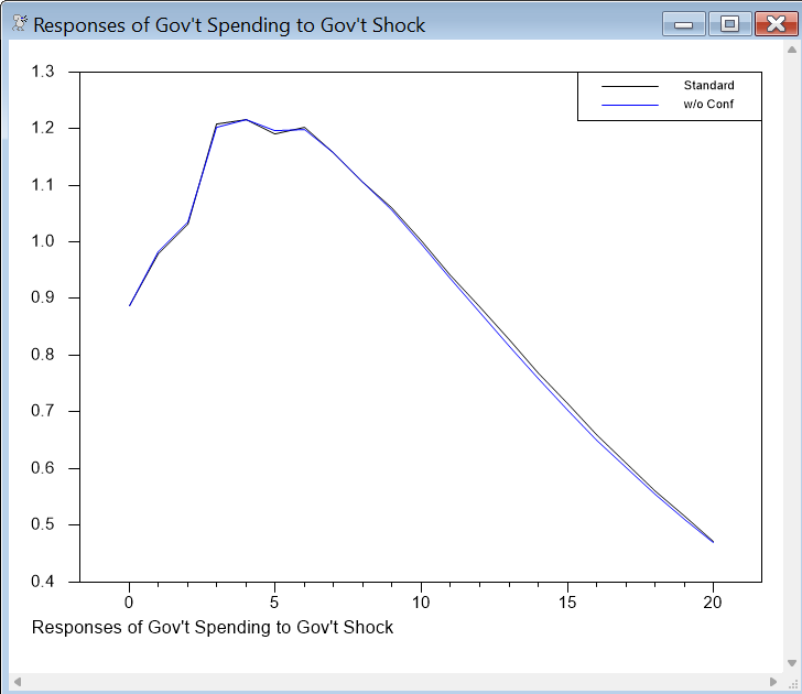
We can now compare graphically the responses to shocks in G using the standard Cholesky shocks (the "1" column in the IRF matrix) with those with the confidence effect shut down (the 1 and only column in the IRF_NOC matrix).

graph(number=0,nodates,footer="Responses of Gov't Spending to Gov't Shock",$

key=upright,klabels=||"Standard","w/o Conf"||) 2

# irf(1,1)

# irf_noc(1,1)

graph(number=0,nodates,footer="Responses of GDP to Gov't Shock",$

key=upright,klabels=||"Standard","w/o Conf"||) 2

# irf(3,1)

# irf_noc(3,1)

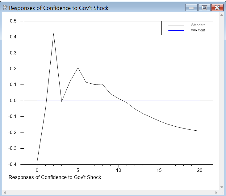
graph(number=0,nodates,footer="Responses of Confidence to Gov't Shock",$

key=upright,klabels=||"Standard","w/o Conf"||) 2

# irf(2,1)

# irf_noc(2,1)

Full Program

cal(q) 1960:1
open data shutdowndata.rat
data(format=rats) / REALGOVT<<'GCEC1' REALGDP<<'GDPC1' CONF<<'UMCSENT' POP<<'CNP16OV'
*
* Convert real quantities to log per capita
*
set lg_pc = 100.0*log(realgovt/pop)
set yg_pc = 100.0*log(realgdp/pop)
set lconf = 100.0*log(conf)
*
system(model=gcy)
variables lg_pc lconf yg_pc
lags 1 to 4
det constant
end(system)
*
estimate
*
* Compute the sequence of own (Cholesky) shocks to confidence to shut down the
* response of confidence to government spending.
*
compute factor=%chol(%sigma)
compute steps=21
impulse(model=gcy,factor=factor,steps=steps,results=irf)
*
dec rect cresp(steps,steps)
ewise cresp(i,j)=%if(j<=i,irf(2,2)(i-j+1),0.0)
dec vect cresptog(steps)
ewise cresptog(i)=-irf(2,1)(i)
compute cshocks=%solve(cresp,cresptog)
*
* Compute the path of shocks which corresponds to that.
*
dec rect cholshocks(steps,3)
compute cholshocks=%unitv(steps,1)~cshocks~%zeros(steps,1)
*
* Use the MATRIX option on IMPULSE to do the response to the unit Cholesky shock
* in government spending with the corresponding confidence shocks to shut out the
* confidence response
*
impulse(model=gcy,steps=steps,matrix=cholshocks*tr(factor),responses=irf_noc)
*
graph(number=0,nodates,footer="Responses of Gov't Spending to Gov't Shock",$
key=upright,klabels=||"Standard","w/o Conf"||) 2
# irf(1,1)
# irf_noc(1,1)
graph(number=0,nodates,footer="Responses of GDP to Gov't Shock",$
key=upright,klabels=||"Standard","w/o Conf"||) 2
# irf(3,1)
# irf_noc(3,1)
graph(number=0,nodates,footer="Responses of Confidence to Gov't Shock",$
key=upright,klabels=||"Standard","w/o Conf"||) 2
# irf(2,1)
# irf_noc(2,1)

Graphs