|
Examples / SWARCH.RPF |
SWARCH.RPF is an example of a Markov switching ARCH model. MS-ARCH was proposed by Hamilton and Susmel(1994), and independently, Cai(1994) as an alternative to a (standard) GARCH model. In these models, instead of the lagged variance term providing the strong connection for volatility from one period to the next, a Markov model governs switches between several variance regimes. Markov Switching GARCH models are much more technically demanding and results with them tend to be suspect.
There are several possible ways to model the effect of the different regimes on volatility: the one used in SWARCH.RPF is from Cai. It multiplies the constant term in the variance equation by a regime-dependent value. Hamilton and Susmel handle it in a slightly different fashion that’s a bit more complicated—see the replication files for that paper.
The series being analyzed are returns on the US/Japan exchange rate.
open data g10xrate.xls
data(format=xls,org=columns) 1 6237 usxjpn
*
set x = 100.0*log(usxjpn/usxjpn{1})
The model is a 3 regime, 2 ARCH lag model. Q=2 sets the ARCH lags; this allows the number of lags to be changed easily. The variance in regime \(i\) at time \(t\) is
\begin{equation} h_t^{(i)} = v^{(i)} a_0 + a_1 u_{t - 1}^2 + a_2 u_{t - 2}^2 \label{eq:swarch_caimodel} \end{equation}
This is an "innovational" model, where the variance doesn't change immediately when moving to a different regime—only the variance intercept changes which affects the model variance gradually since the lagged u's would be from the old regime.
Because the likelihood depends only upon the current regime, we don't need a positive value for LAGS on @MSSETUP.
@MSSetup(regimes=3)
compute q=2
HV will be the relative variances in the regimes (The \(v\) in \eqref{eq:swarch_caimodel}). This will be normalized to a relative variance of 1 in the first regime. The advantage of this (as opposed to just having a separate variance intercept in each regime) is that HV will not be dependent upon the scale of the data—that will be caught by the single parameter \(a_0\) while the \(v\) will be easy to interpret as relative scales.
dec vect hv(nregimes)
This will be the vector of ARCH parameters
dec vect a(q)
We have three parts of the parameter set: the mean equation parameters (here, just an intercept), the ARCH model parameters (with HV(1) pegged to 1), and the Markov switching parameters, for which we’ll use the logistic indexes.
nonlin(parmset=meanparms) mu
nonlin(parmset=archparms) a0 a hv hv(1)=1
nonlin(parmset=msparms) theta
uu and u are used for the series of squared residuals and the series of residuals needed to compute the ARCH variances.
clear uu u
The FUNCTION ARCHRegimeF returns a vector of likelihoods for the various regimes at TIME given residual E. The likelihoods differ in the regimes based upon the values of HV, where the intercept in the ARCH equation is scaled up by HV.
function ARCHRegimeF time e ht
type vector ARCHRegimeF
type real e
type integer time
type vector *ht
*
local integer i j
local real vi
*
dim ARCHRegimeF(nregimes) ht(nregimes)
do i=1,nregimes
compute vi=a0*hv(i)
do j=1,q
compute vi=vi+a(j)*uu(time-j)
end do i
compute ht(i)=vi
compute ARCHRegimeF(i)=%if(vi>0,$
%density(e/sqrt(vi))/sqrt(vi),0.0)
end do i
end
As is typically the case with Markov switching models, there is no global identification of the regimes. By defining a fairly wide spread for HV, we’ll hope that we’ll stay in the zone of the likelihood where regime 1 is low variance, regime 2 is medium and regime 3 is high.
compute hv=||1,10,100||
These are our guess values for the P matrix. We have to invert that (using %MSPLOGISTIC) to get the guess values for the logistic indexes (THETA).
compute p=||.8,.2,.05|.2,.6,.4||
compute theta=%msplogistic(p)
These are the guess values for the other parameters. The ARCH lag parameters are started close to zero, A0 at the series variance. UU is initialized to the unconditional variance.
stats x
compute mu=%mean,a0=%variance,a=%const(0.05)
set uu = %variance
This will hold the regime-specific variances at each time period:
dec series[vect] regimeh
gset regimeh = %zeros(nregimes,1)
We need to keep series of the residual (U) and squared residual (UU). Because the mean function is the same across regimes, we can just compute the residual and send it to ARCHRegimeF, which computes the likelihoods for the different arch variances.
frml logl = u(t)=(x-mu),uu(t)=u(t)^2,$
f=ARCHRegimeF(t,u(t),regimeh(t)),fpt=%MSProb(t,f),log(fpt)
This is needed to make sure everything is fully initialized:
@MSFilterInit
In this case, the 1,3 probability is effectively zero, which causes problems with the estimation. This pegs the THETA(1,3) element to prevent that. In applying this to a different data set, this might (and probably wouldn’t) be necessary.
nonlin(parmset=pegs) theta(1,3)=-50.00
Because we need 2 lags of UU, the estimation starts at 3.
maximize(start=%(p=%mslogisticp(theta),pstar=%msinit()),$
parmset=meanparms+archparms+msparms+pegs,$
method=bfgs,iters=400,pmethod=simplex,piters=10) logl 3 *
@MSSmoothed %regstart() %regend() psmooth
set p1 = psmooth(t)(1)
set p2 = psmooth(t)(2)
set p3 = psmooth(t)(3)
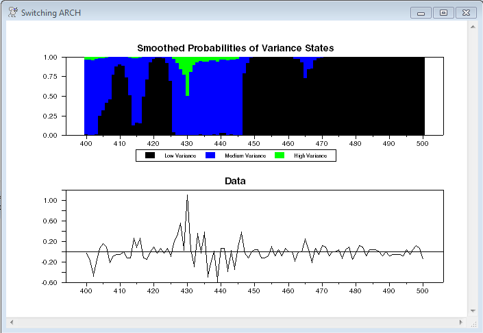
This graphs the smoothed probabilities over a shortened range. Across the full 6237 data points, the graph has too much movement to be usable.
spgraph(vfields=2,samesize,window="Switching ARCH")
graph(style=stacked,maximum=1.0,picture="##.##",$
header="Smoothed Probabilities of Variance States",key=below,$
klabels=||"Low Variance","Medium Variance","High Variance"||) 3
# p1 400 500
# p2 400 500
# p3 400 500
graph(picture="##.##",header="Data")
# x 400 500
spgraph(done)
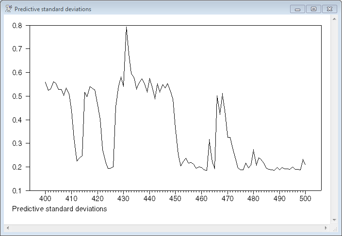
This computes and graphs the predictive standard deviation of the model. This weights the ARCH-predicted variances across regimes by the predicted probabilities.
set predstddev = sqrt(%dot(pt_t1(t),regimeh(t)))
graph(footer="Predictive standard deviations")
# predstddev 400 500
Full Program
open data g10xrate.xls
data(format=xls,org=columns) 1 6237 usxjpn
*
* Convert to percent daily returns
*
set x = 100.0*log(usxjpn/usxjpn{1})
*
* These set the number of regimes, and the number of ARCH lags. Because
* the likelihood depends only upon the current regime, we don't need a
* positive value for LAGS on @MSSETUP.
*
@MSSetup(regimes=3)
compute q=2
*
* HV will be the relative variances in the regimes. This will be
* normalized to a relative variance of 1 in the first regime, so it's
* dimensioned N-1.
*
dec vect hv(nregimes)
*
* This will be the vector of ARCH parameters
*
dec vect a(q)
*
* We have three parts of the parameter set: the mean equation parameters
* (here, just an intercept), the ARCH model parameters, and the Markov
* switching parameters, for which we'll use the logistic indexes.
*
nonlin(parmset=meanparms) mu
nonlin(parmset=archparms) a0 a hv hv(1)=1
nonlin(parmset=msparms) theta
*
* uu and u are used for the series of squared residuals and the series of
* residuals needed to compute the ARCH variances.
*
clear uu u
*
* ARCHRegimeF returns a vector of likelihoods for the various regimes at
* time given residual e. The likelihoods differ in the regimes based upon
* the values of hv, where the intercept in the ARCH equation is scaled
* up by hv.
*
* This is the Cai(1994) model, with the switch on the intercept in the
* variance equation.
*
function ARCHRegimeF time e ht
type vector ARCHRegimeF
type real e
type integer time
type vector *ht
*
local integer i j
local real vi
*
dim ARCHRegimeF(nregimes) ht(nregimes)
do i=1,nregimes
compute vi=a0*hv(i)
do j=1,q
compute vi=vi+a(j)*uu(time-j)
end do i
compute ht(i)=vi
compute ARCHRegimeF(i)=%if(vi>0,$
%density(e/sqrt(vi))/sqrt(vi),0.0)
end do i
end
*
* As is typically the case with Markov switching models, there is no
* global identification of the regimes. By defining a fairly wide spread
* for hv, we'll hope that we'll stay in the zone of the likelihood where
* regime 1 is low variance, regime 2 is medium and regime 3 is high.
*
compute hv=||1,10,100||
*
* These are our guess values for the P matrix. We have to invert that to
* get the guess values for the logistic indexes.
*
compute p=||.8,.2,.05|.15,.6,.4||
compute theta=%msplogistic(p)
*
* These are the guess values for the other parameters. The ARCH lag
* parameters are started close to zero, A0 at the series variance. UU is
* initialized to the unconditional variance.
*
stats x
compute mu=%mean,a0=%variance,a=%const(0.05)
set uu = %variance
*
* This will hold the regime-specific variances at each time period
*
dec series[vect] regimeh
gset regimeh = %zeros(nregimes,1)
*
* We need to keep series of the residual (u) and squared residual (uu).
* Because the mean function is the same across regimes, we can just
* compute the residual and send it to ARCHRegimeF, which computes the
* likelihoods for the different ARCH variances.
*
frml logl = u(t)=(x-mu),uu(t)=u(t)^2,$
f=ARCHRegimeF(t,u(t),regimeh(t)),fpt=%MSProb(t,f),log(fpt)
*
@MSFilterInit
*
* In this case, the 1-->3 probability is effectively zero, which causes
* problems with the estimation. This pegs the theta(1,3) element to
* prevent that. In application to a different data set, this might (and
* probably wouldn't) be necessary.
*
nonlin(parmset=pegs) theta(1,3)=-50.00
*
* Because we need 2 lags of uu, the estimation starts at 3.
*
maximize(start=%(p=%mslogisticp(theta),pstar=%msinit()),$
parmset=meanparms+archparms+msparms+pegs,$
method=bfgs,iters=400,pmethod=simplex,piters=10) logl 3 *
*
@MSSmoothed %regstart() %regend() psmooth
set p1 = psmooth(t)(1)
set p2 = psmooth(t)(2)
set p3 = psmooth(t)(3)
*
spgraph(vfields=2,samesize,window="Switching ARCH")
*
* This graphs the smoothed probabilities over a shortened range. Across
* the full 6237 data points, the graph has too much movement to be
* usable.
*
graph(style=stacked,maximum=1.0,picture="##.##",$
header="Smoothed Probabilities of Variance States",key=below,$
klabels=||"Low Variance","Medium Variance","High Variance"||) 3
# p1 400 500
# p2 400 500
# p3 400 500
graph(picture="##.##",header="Data")
# x 400 500
spgraph(done)
*
* Compute the predictive standard deviation of the model. This weights
* the ARCH predicted variances across regimes by the predicted
* probabilities.
*
set predstddev = sqrt(%dot(pt_t1(t),regimeh(t)))
graph(footer="Predictive standard deviations")
# predstddev 400 500
Output
Statistics on Series X
Observations 6236
Sample Mean 0.014351 Variance 0.398893
Standard Error 0.631580 SE of Sample Mean 0.007998
t-Statistic (Mean=0) 1.794334 Signif Level (Mean=0) 0.072808
Skewness 0.784016 Signif Level (Sk=0) 0.000000
Kurtosis (excess) 13.265486 Signif Level (Ku=0) 0.000000
Jarque-Bera 46362.538224 Signif Level (JB=0) 0.000000
MAXIMIZE - Estimation by BFGS
Convergence in 49 Iterations. Final criterion was 0.0000019 <= 0.0000100
Usable Observations 6235
Function Value -4735.2506
Variable Coeff Std Error T-Stat Signif
************************************************************************************
1. MU -0.0079168 0.0029626 -2.67227 0.00753395
2. A0 0.0050870 0.0006424 7.91823 0.00000000
3. A(1) 0.0464930 0.0185572 2.50538 0.01223184
4. A(2) -0.0042225 0.0004675 -9.03135 0.00000000
5. HV(1) 1.0000000 0.0000000 0.00000 0.00000000
6. HV(2) 30.3185542 3.6361225 8.33816 0.00000000
7. HV(3) 184.8035022 22.4251659 8.24090 0.00000000
8. THETA(1,1) 4.5527742 0.9079920 5.01411 0.00000053
9. THETA(2,1) 2.3741090 0.9644730 2.46156 0.01383339
10. THETA(1,2) -1.6174687 0.2560696 -6.31652 0.00000000
11. THETA(2,2) 2.2003358 0.1817281 12.10785 0.00000000
12. THETA(1,3) -50.0000000 0.0000000 0.00000 0.00000000
13. THETA(2,3) -1.4536927 0.2071508 -7.01756 0.00000000
Graphs
Copyright © 2026 Thomas A. Doan