Example Five: Cross Section Data

For our next example, we will look at a cross sectional data set. This data is taken from Chapter 2 of Verbeek (2008) and is provided on a text file called WAGES1.DAT. The file contains survey data for 3294 young workers, and includes four series: WAGE (hourly wage in dollars), MALE (a 1/0 dummy variable, equal to 1 for male respondents and 0 for female respondents), EXPER (years of experience at work), and SCHOOL (years of schooling). This example is provided on the file ExampleFive.rpf.

Reading the Data

To get started, close the windows from the previous session and do File—New—Editor/Text Window to create a new input window. When you are ready, select the Data/Graphics—(Other Formats) operation and open the file WAGES1.DAT. (you may need to select “Text Files (*.*)” from the list of formats in order to see the file in the dialog box). Click on “Show Preview” (if necessary) to examine the data on the file:

The data run down the page in columns, so the default settings should be correct. When you OK this, you will first be asked

Since this is cross section data, answer "Yes". Next you'll be asked to verify the series names:

Since the series all have valid names, you can just "OK for All". This will generate:

OPEN DATA "wages1.dat"

DATA(FORMAT=PRN,ORG=COLUMNS) 1 3294 EXPER MALE SCHOOL WAGE

The SMPL Option: Selecting Sub-Samples

Our first task is to examine the average wages for both males and females. As noted earlier, the series MALE is equal to 1 for males, and 0 for females. In Example Three, we used the STATISTICS instruction to compute averages (among other basic statistics). But how to compute an average of WAGE using only certain observations (for males only, and for females only)?

The answer is to use the SMPL option (short for sample), which allows you to specify a sub-sample using a logical and/or numeric expression. The syntax is simply

smpl=expression(t)

Observations for which expression(t) returns a logical “true” or a non-zero numeric value are included in the operation. Observations where expression(t) returns a logical “false” or the number 0 are omitted from the operation.

For example:

stats(smpl=male) wage

computes summary statistics for WAGE, using only observations where MALE is 1

Statistics on Series WAGE

Observations 1725 Skipped/Missing 1569

Sample Mean 6.313021 Variance 12.242031

Standard Error 3.498861 SE of Sample Mean 0.084243

t-Statistic (Mean=0) 74.938512 Signif Level (Mean=0) 0.000000

Skewness 1.921402 Signif Level (Sk=0) 0.000000

Kurtosis (excess) 8.845542 Signif Level (Ku=0) 0.000000

Jarque-Bera 6685.148147 Signif Level (JB=0) 0.000000

Using the Statistics—Univariate Statistics operation, the dialog box would look like this:

Most instructions (and associated wizards) that deal with series have the SMPL option.

To get the averages for female workers, you just apply the logical operator .NOT. to the MALE series:

stats(smpl=.not.male) wage

This computes results using only observations where MALE is not equal to 1. This could also be written as:

stats(smpl=male<>1) wage

You could also create a series (using SET or the Transformations wizard) containing the reversed dummy variable and use that for the option. While probably not important here, defining the separate series can make it easier to see what’s happening. If you create a FEMALE series using:

set female = .not.male

you can then use

stats(smpl=female) wage

If you are familiar with certain other statistics program, you might have expected that you would need an “IF” statement to accomplish this. While there is an IF instruction in RATS, it is used to evaluate a single condition, not as an implied loop over a range of observations.

Testing Regression Restrictions

Another way to examine the respective wages for males and females is to regress the WAGE series against a constant and the MALE dummy variable:

linreg wage

# constant male

The coefficient on the CONSTANT will be the average female wage, while the coefficient on the MALE variable will be the difference between male wages and female wages (that is, it reflects the impact of being male on wage). The results show an average female wage of $5.15, with males making an additional $1.17 per hour, for an average of $6.32, with a standard error of $0.11 on the differential.

To determine whether gender truly affects wages earned, Verbeek considers whether other factors, such as years of schooling and years of experience on the job, may explain some or all of the discrepancy. One way to do that is to compare the “restricted regression” used above (restricted because the schooling and experience variables are omitted) with the “unrestricted” regression which does include the additional variables to determine whether the additional components are significant.

RATS offers an instruction specifically for testing these types of exclusion restrictions. Let’s look at the regression with some added factors:

linreg wage

# constant male school exper

You can simply write

exclude

# school exper

This produces the following:

Null Hypothesis : The Following Coefficients Are Zero

SCHOOL

EXPER

F(2,3290)= 191.24105 with Significance Level 0.00000000

The null hypothesis that the added coefficients on schooling and experience are zero (and thus can be excluded from the model) is tested with an F statistic with 2 and 3290 degrees of freedom. The result is significant beyond any doubt, so these variables do seem to help explain wages. However, the regression coefficient on MALE actually goes up in the expanded regression, so the use of the additional factors can’t explain the difference between males and females.

The Regression Test Wizard

You can also generate this test using the Statistics—Regression Tests operation, which displays this dialog box:

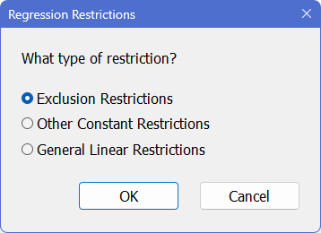
Here, we want to select the “Exclusion Restrictions” option, which tests that some set of coefficients all have zero values. That’s the simplest of the three options.

The “Other Constant Restrictions” is used when you have a test on one or more coefficients with a null hypothesis that they take specific values, not all of which are zero. (A common case, for instance, is that the intercept is zero and a slope coefficient is one).

“General Linear Restrictions” is used when you have restrictions that involve a linear combination of several coefficients (examples are that coefficients sum to one, or coefficients are equal, so their difference is zero).

When you click OK with the “Exclusion Restrictions” on, you get a second dialog box, listing the regressors from that last regression. Select (highlight) the SCHOOL and EXPER series:

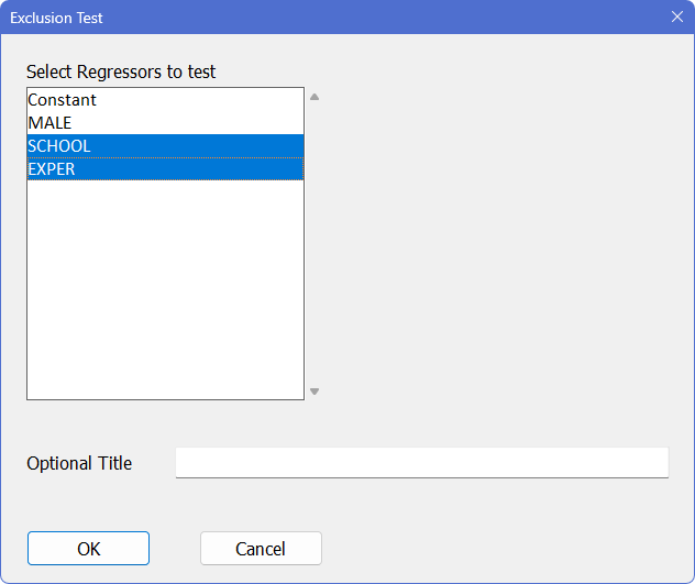
Then click “OK” to run the test. This generates a TEST instruction with a ZEROS option. With TEST, you use numbers rather than variable names to indicate which terms are being tested. In this case, we are testing that the third and fourth regressors in the LINREG are (jointly) zero, so the instruction generated by the wizard is:

TEST(ZEROS)

# 3 4

Learn More: Hypothesis Testing

Chapter 4 of the User’s Guide provides full details on hypothesis testing, including detailed information on the instructions described above, as well as the specialized instructions SUMMARIZE and RATIO. You will also find out how to implement serial correlation and heteroscedasticity tests, Chow tests, Hausman tests, unit root tests, and many more.

X-Y Scatter Plots: The SCATTER Instruction

We’ve looked at creating time series (data vs. time) graphs with GRAPH. You can also graph one series against another to produce a “scatter” or “X–Y” plot.

To demonstrate, let’s look at the relationship between wages earned and years of schooling. First, we will regress WAGE against a constant and SCHOOL, and compute the fitted values from this regression. You can do that using the Statistics—Linear Regressions wizard, adding a series name in the “Fitted Values to” field to save the fitted values, or you can type the instructions directly, using the instruction PRJ (short for project), which computes the fitted values from the most recent regression:

linreg wage

# constant school

prj wagefit

To draw the graph, select Data/Graphics—Scatter (X–Y) Graph to bring up the Scatter Graph wizard.

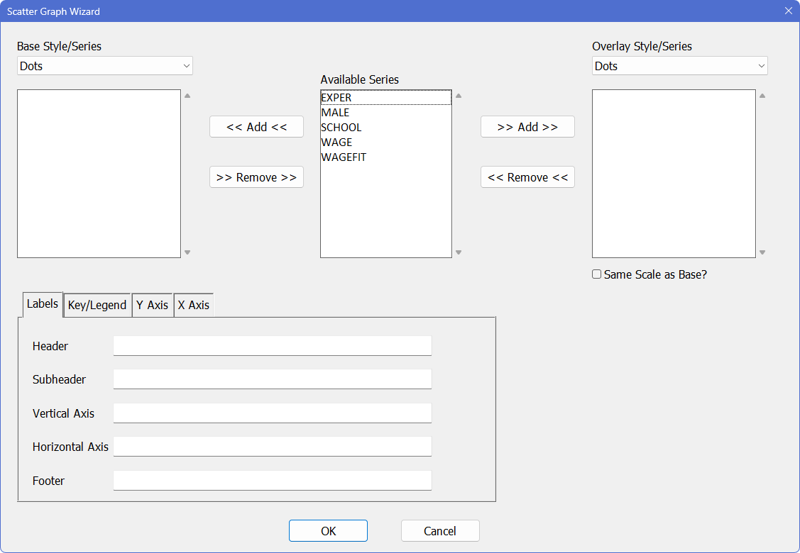
Select (highlight) both WAGE and SCHOOL from the "Available Series" list and click on to add the pair to the list of series to be graphed. (Note that you have to pick two series). When prompted, choose the combination with SCHOOL as the X-axis variable and click “OK”. Then, select “Symbols” as the “Style”.

Now, select WAGEFIT and SCHOOL in "Available Series" and click on the button to add this pair to the “Overlay Series” list. SCHOOL should again be the X-axis variable. Select “Lines” as the "Overlay Style", and turn on the “Same Scale as Base?” switch (we want both pairs of series to be graphed using the same vertical scale).

In the dialog box below, we’ve also added labels for the horizontal and vertical axis:

Clicking “OK” generates the following SCATTER instruction, and the graph shown below:

SCATTER(STYLE=SYMBOLS,OVERLAY=LINES,OVSAME,VLABEL="Hourly Wages",HLABEL="Years of School") 2

# SCHOOL WAGE

# SCHOOL WAGEFIT

As you can see, the OVERLAY option allows us to combine (overlay) two different styles (possibly with two different scales) on a single graph.

Learn More: Comments

If you look at ExampleFive.rpf, you will see, in addition to the instructions that we just generated, lines like the following:

* Adds school and exper to the regression and test the joint

* significance of the two additional variables.

These are comments that we added to explain what’s going on to someone reading the example file, but not following it in this section. It’s generally a good idea to add comments to any program file that you save.

Learn More: Error Messages

In a perfect world, we wouldn’t need to talk about errors or error messages. Unfortunately, you will undoubtedly encounter an occasional error message in your work with RATS. "Error/Warning Messages" discusses how to interpret error messages and fix errors.

Learn More: Entry Ranges

In this example, we have looked at using the SMPL option to control the set of entries to be used in computing a regression. "Entry Ranges" covers the different ways of handling selection of ranges/cases for analysis.

Learn More: Linear Regressions Wizard

You’ll notice that Example Three used only a few features off the Linear Regressions Wizard. We’ll talk a bit here about what else is available:

Robust (HAC) Standard Errors

This is a checkbox which you can use to change the way that the regression standard errors are computed. It won’t change the coefficients; just the standard errors, the covariance matrix, and any regression tests that you do afterwards. If you apply this to our last linear regression in this example, you will get the following instruction:

linreg(robust) wage

# constant school

so you could also simply have inserted the ROBUST option into the existing instruction. If you compare the output, you’ll see a few differences. First, it now says:

Linear Regression - Estimation by Least Squares

With Heteroscedasticity-Consistent (Eicker-White) Standard Errors

so while it still estimates by least squares, the standard errors are now computed using the Eicker-White methods, which are “robust” to certain types of heteroscedasticity (hence the name of the option). If you aren’t familiar with this, see "Linear Regressions: A General Framework". You also might notice that the regression $F$ isn’t shown: that’s a test which is computed under the assumption of homoscedastic errors, and you’ve said (by using the ROBUST option) that that isn’t true. The other summary statistics are the same, as are the coefficients, but the standard errors are (slightly) different, so the T-Stat and Signif columns change as well.

When you click on the “Robust (HAC) Standard Errors” check box, you will also notice that two additional fields below it become active: the “Lags/Bandwidth” and “Lag Window Type”. These aren’t of any special interest in this example, since this is cross section data, but these allow you to compute standard errors which are also robust to autocorrelation (the HAC is short for Heteroscedastic Auto Correlated). If we applied that here (not that we should), the new instruction would be something like:

linreg(robust,lags=3,lwindow=newey) wage

# constant school

Residuals

Further down in the wizard, you will notice a drop down box labeled “Residuals To”. Whenever, you run a regression, RATS creates a series named %RESIDS and fills it with the residuals. If you want to graph the residuals, or compute its statistics, you can just use %RESIDS like any other series. However, if you run a new regression, %RESIDS will now get the residuals from that. If you want to keep a copy of the residuals from one specific regression, you can give a (valid) series name in this box, which will generate the new instruction (see "Entry Ranges" for a description of the /):

linreg wage / u

# constant school

Show Standard Output

This is a checkbox which you will almost always want to be on. If you click it off, you will generate an instruction like this, adding the NOPRINT option:

linreg(noprint) wage

# constant male

Almost all instructions which ordinarily would produce some output will have the option of NOPRINT. Why would you want to do that? Perhaps all you really want from the regression are the residuals. Or the defined equation for forecasting. When you run a regression, almost anything computed by the LINREG is available for further calculations. For instance, the coefficients are in a vector called %BETA; the sum of squared residuals are in %RSS. Perhaps you only need those. If you plan ahead and use NOPRINT, you don’t have to read past the unwanted regression output.

Show VCV of Coefficients

This is a checkbox that you will usually want to be off. If it is on, the estimation instruction will include the VCV option (using the larger regression from the example):

linreg(vcv) wage

# constant male school exper

This places the following below the standard regression output (and puts a similar report into the Window—Report Windows list):

Covariance\Correlation Matrix of Coefficients

Constant MALE SCHOOL EXPER

Constant 0.216203148 -0.15560300 -0.90642459 -0.54623329

MALE -0.007790538 0.011594097 0.09663502 -0.10932520

SCHOOL -0.013822338 0.000341249 0.001075567 0.18093999

EXPER -0.006035400 -0.000279728 0.000141010 0.000564669

This is a square table with covariances on and below the diagonal and correlations above the diagonal. For instance, the estimated variance of the coefficient on MALE (the number at the intersection of the MALE row and MALE column) is roughly .0116. The estimated correlation between the coefficients on MALE and EXPER is where the MALE row and the EXPER column meet (above the diagonal), roughly -0.109. The covariance of the same two coefficients is at the EXPER row and MALE column (-.00028). Note that the header says "Covariance\Correlation". We use the \ to help you remember the structure of the matrix: covariance below and correlation above.

We recommend that you not use this on a regular basis simply because there is little useful information in it. The covariances are used in doing joint hypothesis tests as above, but you will be using instructions like TEST and EXCLUDE that do the computations for you, rather than using numbers out of this table.

The Method Popup Box

Everything we have done so far has used the (default) choice of “Least Squares” in the “Method” box at the top left. There are several other choices available, some of which generate LINREG with a different set of options; others generate different instructions with a similar overall look to LINREG.

The next two choices are “Two Stage Least Squares” and “GMM (IV with Optimal Weights)”. If you choose one of those, you’ll notice that the “Instruments” box and button become enabled. These are (closely related) instrumental variables estimation methods which require both a list of regressors and a list of instruments. You add variables to the instruments list just as you do for the regressors: you can either type them directly into the box, or you can use the button to pop up a dialog box to manage the list. If we choose “Two Stage Least Squares”, and use CONSTANT and SCHOOL as the Explanatory Variables and CONSTANT, EXPER and MALE as the Instruments, we generate the instructions:

instruments constant exper male

linreg(inst) wage

# constant school

The instruments are listed on the separate INSTRUMENTS instruction line. That allows you to do several LINREG’s off the same list without having to re-enter the instrument information. Two-stage least squares is done by adding the INST (short for INSTRUMENT) option to LINREG.

The next two choices for the “Method” box are “AR(1) Regression” and “AR(1)-Instrumental Variables”. These will generate a different instruction: AR1, which is for linear regressions with first-order autocorrelated errors. We won’t look further at this here, but would like to point out that parts of the dialog change when you choose this (and all the remaining methods). In particular, the “Robust (HAC) Standard Errors” is replaced by a different popup box for the “AR1 Method”.

The next choice down on the “Method” box is “Robust Regression”, which generates an RREG (Robust REGression) instruction. This is still a linear regression, but uses a different estimation technique which is more “robust” to outliers.

The final choice is “Stepwise Regression”, which generates an STWISE instruction. Stepwise regression is nowhere near as popular as it was perhaps thirty years ago, but still has its place. If you’re interested in this, see the description of STWISE.

Other Related Instructions

There are several other instructions which have similarities in form to LINREG, in the sense that the instruction looks like:

instruction(options) dependent_variable start end

# list of explanatory variables

but have option sets that are so different that they can’t easily be fit into the same wizard. These are the next several choices on the Statistics menu:

The Limited/Discrete Dependent Variables wizard handles the DDV (Discrete Dependent Variables) and LDV (Limited Dependent Variables) instructions. DDV is used for techniques applied to data where the dependent variable is “discrete” (usually just values 0 and 1) such as logit and probit. LDV is used for techniques such as tobit which are applied when the dependent variable is continuous, but the observed range is somehow limited. These are covered in "Cross Section Data Methods".

The Panel Data Regressions wizard generates a PREGRESS instruction, which includes special techniques for estimating the linear regression with panel data (often also known as longitudinal or cross section-time series data); techniques such as fixed effects and random effects. These are covered in "Panel and Grouped Data".

The Recursive Least Squares wizard generates an RLS instruction. When applied over the same range as a LINREG, it will give exactly the same output—the point is that it does a whole set of calculations for reduced ranges that can be used to check for stability in the overall linear model. See
"Recursive Least Squares".

There are quite a few other estimation instructions, but they have quite a different form. The instructions included here have models which are based upon a linear combination of a set of explanatory variables. If we need a non-linear function, we will need a different way to enter that than just a list of variables. We’ll see one of these other instructions (NLLS, for non-linear least squares) in Example Six.

There are several other instructions which apply to systems of linear equations rather than just single equations: SUR ("Systems Estimation: Linear"), which does fairly general systems, and ESTIMATE, which estimates the equations of a Vector AutoRegression (VAR).