Diebold Yilmaz IJF 2012

This is a description of the specific analysis done in the replication for Diebold and Yilmaz(2012). There's a separate page for the earlier Diebold and Yilmaz(2009). See "Diebold Yilmaz spillover papers" for a description of the common structure of the programs and analysis.

The 2012 paper replaces the Cholesky factorization with the "generalized" one. How you choose between them is described on the "Spillover Papers" page. It is applied to a much smaller set of series (four rather than nineteen), which allows for some extra calculations. There are two program files provided:

dyijf2012.rpf

Creates the full-sample "spillover" table for the volatility measures and the rolling sample estimates.

dyijf2012_sensitivity.rpf

Does the sensitivity analysis (to either lag length in the VAR or to the horizon) from their appendix.

These programs make use of the HASH aggregator. This defines a short label (for tables) and a long label (for graphs) for each of the four series.

dec hash[string] shorthash longhash

compute shorthash("sp500")="Stocks",$

longhash("sp500")="Stock market – S&P 500 Index"

compute shorthash("r_10y")="Bonds",$

longhash("r_10y")="Bond Market – 10-year Interest Rate"

compute shorthash("djubscom")="Commodities",$

longhash("djubscom")="Commodity Market – DJ/UBS Index"

compute shorthash("usdx")="FX",$

longhash("usdx")="FX Market – US Dollar Index Futures"

The advantage of doing this (rather than directly creating VECT[STRINGS] for the different labels as is done in the replication for the 2009 paper) is seen when we create the VECT[STRINGS] (later) for handling the labels:

dec vect[string] shortlabels(%nvar) longlabels(%nvar)

ewise shortlabels(i)=shorthash(%l(%modeldepvars(assetvar)(i)))

ewise longlabels(i)=longhash(%l(%modeldepvars(assetvar)(i)))

This pulls the labels (%L function) of the dependent variables (%MODELDEPVARS function) from the VAR model. %MODELDEPVARS returns a VECTOR of the series handles, so we add an I subscript to take the element i out of that. Since we used the variable names as the "keys" for the HASH, this will give us the strings associated with a particular series. If we were experimenting with different variables in the VAR, we could add the labels for each to the shorthash and longhash and the working labels would automatically adapt to the chosen set of variables. (This isn't important here, where we don't make changes like that, but would be useful in actual practice where you might).

This section does graphs of the annualized volatilities. Note that these graphs and the use of logs is specific to the data being daily volatility estimates.

spgraph(vfields=2,hfields=2,$

header="Figure 1. Daily U.S. Financial Market Volatilities",$

subheader="Annualized Standard Deviation, Percent")

dofor i = sp500 r_10y djubscom usdx

set ann_std_dev = 100*sqrt(365*i{0})

graph(header=longhash(%l(i)))

# ann_std_dev

end dofor i

spgraph(done)

dofor i = sp500 r_10y djubscom usdx

set i = log(i{0})

end do i

The rolling sample analysis adds several calculations that aren't included in the 2009 paper:

1.Directional spillover measures "From Others" for each the four series

2.Directional spillover measures "To Others" for each of the four series

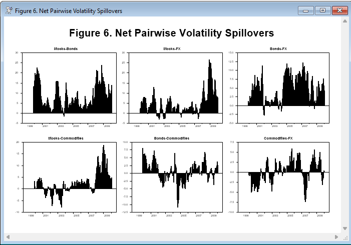
3.Net Pairwise spillovers between each pair of series.

In the full-sample table of results:

Stocks Bonds Commodities FX From Others

Stocks 88.76 7.29 0.35 3.61 11.2

Bonds 10.21 81.45 2.73 5.61 18.6

Commodities 0.47 3.70 93.69 2.14 6.3

FX 5.69 7.03 1.55 85.73 14.3

Contribution to others 16.4 18.0 4.6 11.4 50.4

Contribution including own 105.1 99.5 98.3 97.1 12.6%

the "From Others" and "To Others" (sums across rows and down columns, not including the diagonal) are those statistics computed separately for each rolling sample. The net pairwise spillovers are the differences between (i,j) and (j,i) values (thus depend for sign upon the order in which they are computed).

These are all computed in parallel. The setup is

dec series totalspill

dec symm pairvar(%nvar,%nvar)

dec vect[series] fromspill(%nvar) tospill(%nvar) netspill(%nvar)

dec symm[series] pairspill(%nvar,%nvar)

clear(zeros) fromspill topspill totalspill netspill pairspill

(PAIRSPILL is set up as SYMMETRIC for convenience, but the diagonals are zeros), and the working code is

compute gfevdx=%xt(gfevd,nsteps)

ewise tovar(i)=%sum(%xcol(gfevdx,i))-gfevdx(i,i)

ewise fromvar(i)=%sum(%xrow(gfevdx,i))-gfevdx(i,i)

ewise pairvar(i,j)=gfevdx(i,j)-gfevdx(j,i)

compute totalspill(end)=100.0*%sum(tovar)/%nvar

compute %pt(fromspill,end,100.0*fromvar)

compute %pt(tospill,end,100.0*tovar)

compute %pt(netspill,end,100.0*(tovar-fromvar))

compute %pt(pairspill,end,100.0*pairvar)

which saves information in each at entry END, which is the end point in the rolling sample. The %PT function is used to store information from a VECTOR or SYMMETRIC into a particular set of slots in a VECTOR or SYMMETRIC of SERIES.

The various graphs done in this paper can get fairly complicated to lay out if you have a different number of series. Figures 3, 4 and 5 all need one graph pane per series (which is either the source or the target for spillover). This is designed to handle any number of series, though the graphs get cluttered about about six:

compute rows=fix(sqrt(%nvar))

compute cols=(%nvar-1)/rows+1

spgraph(vfields=rows,hfields=cols,$

header="Figure 3. Directional Volatility Spillovers, FROM Four Asset Classes")

do i=1,%nvar

graph(header=longlabels(i),style=bar)

# fromspill(i) rstart+nspan-1 rend

end do i

spgraph(done)

The ROWS and COLS compute the number of rows and columns that will give the best looking graph for %NVAR panes and is used for Figures 3, 4 and 5.

Figure 6 does pairwise combinations. Note that the number of those (PAIRTOTAL below) can get very big, very fast. With more than 5 series, you would probably be better off doing one separate graph for each target series with all the others.

compute pairTotal=(%nvar-1)*%nvar/2

compute pairRows=fix(sqrt(pairTotal))

compute pairCols=(pairTotal-1)/pairRows+1

spgraph(vfields=pairRows,hfields=pairCols,$

header="Figure 6. Net Pairwise Volatility Spillovers")

do i=1,%nvar

do j=i+1,%nvar

graph(header=shortlabels(i)+"-"+shortlabels(j),style=bar)

# pairspill(i,j)

end do j

end do i

spgraph(done)