Dueker JBES 1997

Dueker(1997) was one of two papers (the other is Gray(1996)) written in the mid 1990's proposing methods of implementing Markov Switching GARCH (MS-GARCH) models. Because the GARCH recursion depends upon the unobservable lagged variance (unlike an ARCH, which requires only observable lagged residuals), the exact analysis of MS-GARCH is infeasible as the variance depends upon the entire past history of the regimes. Dueker and Gray proposed different methods for collapsing the information in past regimes down to a manageable level. Unfortunately, Dueker's application to stock market returns was generally unsuccessful in finding any real split in regimes, even though his filtering method was probably superior to Gray's. A detailed comparison of the Dueker and Gray filters and an application of Dueker's filter to a more appropriate data set is included in the Structural Breaks and Switching Models e-course.

All of the models have a mean only as the mean model, and all use conditionally Student-t distributed errors. Neither is required to use the Dueker filter. The paper does five different MS-GARCH models with different choices for which parameters are allowed by switch between regimes and none of Dueker's models allows all covered parameters to switch with the regime. (Again, this is the author's choice, and isn't required to use his filter).

dueker_swarch.rpf

This does the simpler switching ARCH, which has a log likelihood which can be computed exactly.

dueker_swgarch.rpf

This allows only the means to switch, which is accomplished by constraining the variances to be equal through the parameter set:

nonlin(parmset=fixgv) gv(2)=gv(1)

Even though the parameters which directly govern the variance process are fixed between regimes, the current variance still depends upon the entire history of the regimes because of the (regime-dependent) lagged squared residuals which then creates regime-dependence in the lagged variance through the GARCH recursion.

dueker_swgarch_nf.rpf

This allows both switching means and GARCH normalization (scale) factors.

dueker_swgarch_uv.rpf

This allows both switching means and GARCH model intercepts.

dueker_swgarch_df.rpf

This allows both switching means and degrees of freedom of the t distributions. Because there is very little difference in the t density once you get above (roughly) 50 degrees of freedom, the two degrees of freedom parameters are capped at 50 using

nonlin(parmset=limit) nuv(1)<=50.0 nuv(2)<=50.0

dueker_swgarch_k.rpf

The means and the degrees of freedom of the t distributions switch, but the variances themselves are fixed. This is different from the dueker_swgarch_df.rpf example where the GARCH recursion is fixed, but computes the variance of the numerator Normal in the t distribution, rather than the variance of the t distribution itself.

None of the models does well enough with this data set to conclude that the added complication is worth it. A fixed regime GARCH with t errors has a log likelihood of -3312.7305. The best of the five MS-GARCH models is the "K" model with -3303.1719 but that has regimes which aren't persistent, which makes it likely that the filter approximation isn't working properly. Of the others, the "UV" model is best at -3304.0253, but that has nine parameters compared with five in the fixed regime GARCH model. With 2527 data points, the simpler model would be strongly preferred using SBC.

Output (from dueker_swgarch_uv.rpf)

This has output from (in order) least squares, a standard (fixed-regime) GARCH model with conditionally t errors and a MS-GARCH model with different means (MU(1) and MU(2)) and variance recursion intercepts (GV(1) and GV(2)) in the two regimes. P(1,1) is the probability of staying in regime 1 and P(1,2) is the probability of moving to 1 from 2 (thus the probability of staying in 2 is 1-0.002464522).

Linear Regression - Estimation by Least Squares

Dependent Variable Y

Usable Observations 2529

Degrees of Freedom 2528

Centered R^2 -0.0000000

R-Bar^2 -0.0000000

Uncentered R^2 0.0019364

Mean of Dependent Variable 0.0484295340

Std Error of Dependent Variable 1.0997180381

Standard Error of Estimate 1.0997180381

Sum of Squared Residuals 3057.3120419

Log Likelihood -3828.3866

Durbin-Watson Statistic 1.9063

Variable Coeff Std Error T-Stat Signif

************************************************************************************

1. Constant 0.0484295340 0.0218678927 2.21464 0.02687358

GARCH Model - Estimation by BFGS

Convergence in 23 Iterations. Final criterion was 0.0000000 <= 0.0000100

Dependent Variable Y

Usable Observations 2527

Log Likelihood -3312.7305

Variable Coeff Std Error T-Stat Signif

************************************************************************************

1. Mean(Y) 0.0551106754 0.0171114122 3.22070 0.00127879

2. C 0.0224917997 0.0065971958 3.40930 0.00065131

3. A 0.0345690992 0.0078553734 4.40069 0.00001079

4. B 0.9397470710 0.0125132322 75.10027 0.00000000

5. Shape 5.3378256984 0.5604269971 9.52457 0.00000000

MAXIMIZE - Estimation by BFGS

Convergence in 58 Iterations. Final criterion was 0.0000098 <= 0.0000100

Usable Observations 2527

Function Value -3304.0253

Variable Coeff Std Error T-Stat Signif

************************************************************************************

1. MU(1) -0.104543765 0.121143628 -0.86297 0.38815193

2. MU(2) 0.061871475 0.016958665 3.64837 0.00026391

3. MSG(1) 0.013332432 0.005112036 2.60805 0.00910604

4. MSG(2) 0.957380672 0.011345127 84.38695 0.00000000

5. GV(1) 0.110260810 0.032764781 3.36522 0.00076482

6. GV(2) 0.019122375 0.006138488 3.11516 0.00183845

7. NU 5.666155473 0.612290057 9.25404 0.00000000

8. P(1,1) 0.973096607 0.017859326 54.48675 0.00000000

9. P(1,2) 0.002464522 0.001587554 1.55240 0.12056612

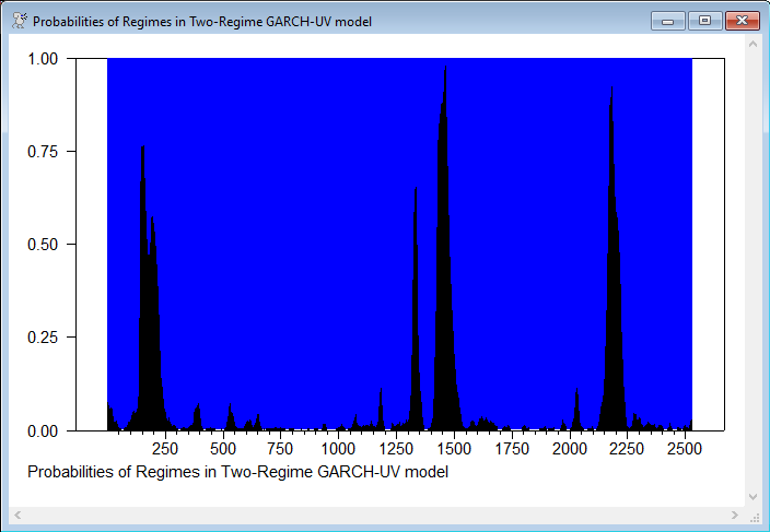
Graph

This is the graph of smoothed probabilities of the regimes from the dueker_swgarch_uv.rpf program. Black is the probability of regime 1 (which is the low mean/high variance regime).