Ehrmann Ellison Valla EL 2003

This is from Ehrmann, Ellison and Valla(2003), which does a 3 variable Markov Switching VAR aimed at studying changes to oil price variances. This is studied in detail in the Structural Breaks and Switching Models e-course.

This has three separate programs:

eev_ml.rpf

estimates the model by maximum likelihood. This is rather slow and ends up finding a local mode.

eev_em.rpf

estimates the model by EM. This is quite a bit faster than eev_ml.rpf and finds a somewhat better mode. (There's no way to no for certain if it's global, but it probably is).

eev_mcmc.rpf

estimates the model by Markov Chain Monte Carlo methods (Gibbs sampling). This is, by far, the most complicated of the three. It's the only one which computes the regime-specific impulse response functions, as it's the only one of the three methods which is able to produce error bands for them. (The other two estimation techniques can be used to generate point estimates of IRF's from their point estimates for the coefficients). Note that the authors used bootstrapping rather than Gibbs sampling to get error bands—Gibbs sampling seems to be a more straightforward approach.

The VAR is monthly data on log capacity utilization, log of the overall price level and log of the oil price. (All are actually 100*log(x) to make interpretation of responses simpler).

@VARLagSelect with the Hannan-Quinn criterion selects 3 lags. This type of MS-VAR is most easily analyzed using @MSSysRegression, which is set up with two regimes, three lags of each variable plus a CONSTANT, with all coefficients plus covariances switching:

@varlagselect(Lags=6,crit=hq)

# logcutil logcpi logpoil

system(model=varmodel)

variables logcutil logcpi logpoil

lags 1 to 3

det constant

end(system)

@mssysregression(model=varmodel,regimes=2,switch=ch)

Note that while the intention is to get regimes to reflect differences in the variance of oil price shocks, there is nothing in the model to force that to be the case. There are 30 regression coefficients and 6 free parameters in the covariance matrix in each regime and changes to any combination of them could end up producing a likelihood-maximizer in a Markov Switching model. Fortunately, in practice, you're more likely to get changes in variance to be the global mode than coefficient changes, so starting out with the goal of finding variance switches is more promising than starting out hoping for interpretable coefficient switches.

In total, this model has 74 total free parameters (30 regression coefficients and 6 covariance matrix parameters in each regime, plus 2 governing the transition probabilities). That's quite a few parameters to estimate using "variational" methods (such as BFGS) which basically treat the function like a "black box". A Markov Switching systems regression in fact has quite a bit of structure, and the most efficient way to estimate it is to use EM (Expectations-Maximization). The implementation of EM for this type of model allows the vast majority of the parameters to be estimated using a probability-weighted linear systems regression. While this has to be re-done with each iteration, this is substantially more efficient than almost blindly trying to play with the individual parameters.

eev_em.rpf

This estimates the model by least squares to help with the initialization of regimes. The regimes are "guessed" to be 1 or 2 based upon values of standardized residuals for oil (3rd variable, where OILPOS=3) in the VAR.

estimate(model=MSSysRegModel,resids=varres)

compute gstart=%regstart(),gend=%regend()

gset MSRegime = $

%if(abs(varres(oilpos))/sqrt(%sigma(oilpos,oilpos))<1.0,1,2)

Those guesses are then used to produce the initial values of the regression coefficients and (more important) covariance matrices. There's no guarantee that the optimum will have regimes that break based upon the oil price shock variances, but this gives you a good chance of finding the optimum if that does turn out to be the case. Note: MSRegime is a SERIES[INTEGER] created by all of the MS procedures—that's why a GSET is used rather than SET. The regimes need to be numbered starting at 1.

@MSSysRegInitial(guess=MSRegime) gstart gend

The estimation with EM is done fairly easily with:

@MSSysRegEMGeneralSetup

do emits=1,50

@MSSysRegEMStep gstart gend

disp "Iteration" emits "Log likelihood" %logl

end do emits

Unfortunately, while this rather quickly gets to an optimum (and an optimum with a large difference in the oil price shock variance between the two regimes), EM, by its nature, doesn't give standard error estimates for the parameters. The recommended procedure is to then "polish" the estimates with 10 iterations of BHHH. You don't want to use BFGS here because the parameters are already converged, so BFGS won't be able to get a good estimate of the curvature (to get standard errors).

This sets up the parameter set using the variables constructed by @MSSysRegression. BETASYS and SIGMAV are specify to the systems regression (BETASYS for the regression coefficients and SIGMAV for the covariance matrices), while P is standard to any of the Markov Switching procedures.

@MSSysRegParmset(parmset=regparms)

nonlin(parmset=msparms) p

In the next segment, the first step truncates the "P" matrix to remove the bottom row since that's the form used for ML estimation. (EM uses the whole matrix, since it just computes that in one part of a "maximization" step). At each time period, %MSSysRegFVec computes the VECTOR of (non-logged) likelihoods, %MSProb does all the Bayes' formula updates given that and returns the (again, non-logged) likelihood. The LOGL FRML then returns the log of that value as the function value for the entry.

The MAXIMIZE uses a START option to let %MSSysRegInit() compute the ergodic (stationary) probabilities and puts those into PSTAR, which is used by the MS procedures to hold the current "filtered" probabilities of the regimes.

compute p=%xsubmat(p,1,1,1,2)

frml logl = f=%MSSysRegFVec(t),fpt=%MSProb(t,f),log(fpt)

maximize(start=(pstar=%MSSysRegInit()),parmset=regparms+msparms,$

method=bhhh,iters=10) logl gstart gend

This shows the output from the EM step (which just traces the log likelihoods) and from the BHHH final estimates. Note that the BHHH intentionally doesn't converge—there's no real advantage to that since (unlike BFGS) the covariance matrix won't really change much from iteration to iteration. Also note that the BHHH log likelihood is slightly better (in this case) than the EM log likelihood. EM actually computes the log likelihood slightly differently (because of how the initial values for the regime probabilities are done) so there will always be a very slight difference, which can go in either direction.

Iteration 1 Log likelihood -1260.92853

Iteration 2 Log likelihood -1198.13645

Iteration 3 Log likelihood -1169.06832

Iteration 4 Log likelihood -1159.42407

Iteration 5 Log likelihood -1154.24922

Iteration 6 Log likelihood -1153.38713

Iteration 7 Log likelihood -1153.31442

Iteration 8 Log likelihood -1153.31141

Iteration 9 Log likelihood -1153.31141

Iteration 10 Log likelihood -1153.31147

Iteration 11 Log likelihood -1153.31149

...

Iteration 49 Log likelihood -1153.31151

Iteration 50 Log likelihood -1153.31151

MAXIMIZE - Estimation by BHHH

NO CONVERGENCE IN 10 ITERATIONS

LAST CRITERION WAS 0.0000000

Monthly Data From 1973:04 To 2000:12

Usable Observations 333

Function Value -1153.2721

Variable Coeff Std Error T-Stat Signif

************************************************************************************

1. BETASYS(1)(1,1) 1.3025018 0.0966859 13.47147 0.00000000

2. BETASYS(1)(2,1) -0.1184801 0.1551684 -0.76356 0.44513065

3. BETASYS(1)(3,1) -0.2301416 0.0971064 -2.36999 0.01778834

4. BETASYS(1)(4,1) -0.0712861 0.4861219 -0.14664 0.88341426

5. BETASYS(1)(5,1) -0.3441576 0.7052440 -0.48800 0.62555132

6. BETASYS(1)(6,1) 0.4326661 0.4004606 1.08042 0.27995472

7. BETASYS(1)(7,1) 0.0322534 0.0712970 0.45238 0.65099485

8. BETASYS(1)(8,1) -0.0128712 0.1151107 -0.11182 0.91096926

9. BETASYS(1)(9,1) -0.0303329 0.0685360 -0.44258 0.65806736

10. BETASYS(1)(10,1) 16.1171711 12.1435052 1.32723 0.18443406

11. BETASYS(1)(1,2) -0.0042298 0.0381574 -0.11085 0.91173330

12. BETASYS(1)(2,2) 0.0567823 0.0561936 1.01048 0.31226685

13. BETASYS(1)(3,2) -0.0299722 0.0281244 -1.06570 0.28655914

14. BETASYS(1)(4,2) 1.1110915 0.1226603 9.05828 0.00000000

15. BETASYS(1)(5,2) 0.0076857 0.1463613 0.05251 0.95812071

16. BETASYS(1)(6,2) -0.1331041 0.1033310 -1.28813 0.19769981

17. BETASYS(1)(7,2) 0.0203414 0.0172547 1.17889 0.23844077

18. BETASYS(1)(8,2) -0.0069076 0.0273464 -0.25260 0.80058112

19. BETASYS(1)(9,2) -0.0056940 0.0152100 -0.37436 0.70813872

20. BETASYS(1)(10,2) -5.5079240 3.8261806 -1.43954 0.14999877

21. BETASYS(1)(1,3) -0.1359305 0.2128054 -0.63876 0.52298229

22. BETASYS(1)(2,3) 0.1406804 0.3341148 0.42105 0.67371568

23. BETASYS(1)(3,3) -0.0018366 0.2046396 -0.00897 0.99283914

24. BETASYS(1)(4,3) 1.9101624 0.9360367 2.04069 0.04128147

25. BETASYS(1)(5,3) -1.4219866 1.0299190 -1.38068 0.16737795

26. BETASYS(1)(6,3) -0.4268509 0.8357095 -0.51076 0.60951587

27. BETASYS(1)(7,3) 1.1247632 0.1221871 9.20525 0.00000000

28. BETASYS(1)(8,3) -0.0311582 0.1915569 -0.16266 0.87078804

29. BETASYS(1)(9,3) -0.1288451 0.1205220 -1.06906 0.28504318

30. BETASYS(1)(10,3) -18.4432940 29.8566941 -0.61773 0.53675513

31. BETASYS(2)(1,1) 1.0099719 0.0786500 12.84135 0.00000000

32. BETASYS(2)(2,1) 0.0757769 0.1184549 0.63971 0.52236023

33. BETASYS(2)(3,1) -0.1289917 0.0815790 -1.58119 0.11383525

34. BETASYS(2)(4,1) 0.4351118 0.4084667 1.06523 0.28677098

35. BETASYS(2)(5,1) -1.6477606 0.6487385 -2.53995 0.01108697

36. BETASYS(2)(6,1) 1.2104123 0.5067981 2.38835 0.01692412

37. BETASYS(2)(7,1) 0.0047449 0.0053218 0.89160 0.37260985

38. BETASYS(2)(8,1) -0.0151109 0.0080892 -1.86803 0.06175851

39. BETASYS(2)(9,1) 0.0078826 0.0049171 1.60308 0.10891595

40. BETASYS(2)(10,1) 21.0452145 9.6384022 2.18348 0.02900082

41. BETASYS(2)(1,2) -0.0058633 0.0153751 -0.38135 0.70294499

42. BETASYS(2)(2,2) -0.0109034 0.0199546 -0.54641 0.58478179

43. BETASYS(2)(3,2) 0.0260421 0.0131540 1.97979 0.04772704

44. BETASYS(2)(4,2) 1.0624433 0.0709570 14.97306 0.00000000

45. BETASYS(2)(5,2) -0.1426209 0.0974345 -1.46376 0.14325911

46. BETASYS(2)(6,2) 0.0752892 0.0548892 1.37166 0.17017027

47. BETASYS(2)(7,2) 0.0017384 0.0008791 1.97738 0.04799906

48. BETASYS(2)(8,2) -0.0018626 0.0013142 -1.41722 0.15641910

49. BETASYS(2)(9,2) 0.0008719 0.0007719 1.12957 0.25865920

50. BETASYS(2)(10,2) -1.5828601 1.1938910 -1.32580 0.18490611

51. BETASYS(2)(1,3) 1.5432515 1.5792307 0.97722 0.32846162

52. BETASYS(2)(2,3) -0.8768512 2.0595459 -0.42575 0.67029017

53. BETASYS(2)(3,3) -0.8624865 1.2961518 -0.66542 0.50578135

54. BETASYS(2)(4,3) -0.1045067 7.4597585 -0.01401 0.98882248

55. BETASYS(2)(5,3) 19.3910528 11.4624206 1.69171 0.09070193

56. BETASYS(2)(6,3) -19.1875197 6.9773537 -2.74997 0.00596006

57. BETASYS(2)(7,3) 1.0983810 0.0702989 15.62444 0.00000000

58. BETASYS(2)(8,3) -0.1761646 0.0917278 -1.92051 0.05479306

59. BETASYS(2)(9,3) -0.0439301 0.0641593 -0.68470 0.49353099

60. BETASYS(2)(10,3) 66.8447170 179.1300609 0.37316 0.70902711

61. SIGMAV(1)(1,1) 0.7747708 0.0905635 8.55500 0.00000000

62. SIGMAV(1)(2,1) 0.0335175 0.0315907 1.06099 0.28869338

63. SIGMAV(1)(2,2) 0.0539895 0.0070497 7.65846 0.00000000

64. SIGMAV(1)(3,1) 0.2189912 0.1601335 1.36755 0.17145185

65. SIGMAV(1)(3,2) 0.0585223 0.0498984 1.17283 0.24086406

66. SIGMAV(1)(3,3) 3.2731541 0.3523026 9.29075 0.00000000

67. SIGMAV(2)(1,1) 0.2857325 0.0351317 8.13317 0.00000000

68. SIGMAV(2)(2,1) -0.0011356 0.0041482 -0.27374 0.78428095

69. SIGMAV(2)(2,2) 0.0079367 0.0009470 8.38100 0.00000000

70. SIGMAV(2)(3,1) -0.3336294 0.4603887 -0.72467 0.46865512

71. SIGMAV(2)(3,2) 0.1333017 0.0694924 1.91822 0.05508309

72. SIGMAV(2)(3,3) 93.4450870 9.5924869 9.74149 0.00000000

73. P(1,1) 0.9732715 0.0163812 59.41402 0.00000000

74. P(1,2) 0.0176582 0.0190685 0.92604 0.35442354

BETASYS(s)(i,j) is the VAR coefficient in regime s, for equation j, coefficient i. VAR coefficients are grouped by variable, so BETASYS(1)(1,1) is the coefficient in regime 1 (low variance regime), coefficient 1 (lag 1 on LOGCUTIL) in equation 1 (on LOGCUTIL), while BETASYS(2)(8,3) is the coefficient in regime 2 (high variance regime), coefficient 8 (lag 2 on the third variable, which is LOGPOIL) and equation 3 (for the third variable, LOGPOIL). Note, however, that these coefficients, like any VAR lag coefficients, are almost impossible to interpret individually, which is why they are almost never reported in published work.

SIGMAV(s)(i,j) is a lot simpler: SIGMAV(s) is the covariance matrix in regime s, with i,j giving the subscripts within it. SIGMAV(1)(3,3) and SIGMAV(2)(3,3) are the estimates of the variance of the oil shock in the two regimes, and they are (as was hoped) quite a bit different.

eev_ml.rpf

This estimates by BFGS, which, as was described earlier, is much slower than EM because it doesn't take advantage of the (largely) linear structure of the model. Rather than using the "guess regimes", this uses the standard guess values and adjusts them to push the regimes toward low variance-high variance on oil. Maximum likelihood (more than EM) can run into problems with spikes in the log likelihood at singularities in the covariance matrix (this is discussed in the Structural Breaks and Switching Models e-course). The REJECT option is set up to throw out any parameter values that have the log determinant of one of the regimes too small to be reasonable.

@mssysregparmset(parmset=regparms)

nonlin(parmset=msparms) p

compute gstart=1973:4,gend=2000:12

@MSSysRegInitial gstart gend

* Reset the 2nd covariance matrix to make regime 2 have a high

* variance for oil.

compute sigmav(2)=%diag(%xdiag(sigmav(1)).*||.25,.25,4.0||)

compute logdetlimit=%MSSysRegInitVariances()-12.0*3

frml logl = f=%MSSysRegFVec(t),fpt=%MSProb(t,f),log(fpt)

@MSFilterInit

maximize(start=$

%(logdet=%MSSysRegInitVariances(),pstar=%MSSysRegInit()),$

parmset=regparms+msparms,reject=logdet<logdetlimit,$

method=bfgs,iters=1000,pmethod=simplex,piters=5) logl gstart gend

eev_mcmc.rpf

This estimates the model by Gibbs sampling. The parameter blocks are:

1.The covariance matrices, which are sampled given the regimes and coefficients (regime-specific residuals being the only statistics required from the coefficients). To prevent the covariance matrices from (possibly) collapsing to singular matrices (if the number of observations in a regime is small), these are drawn using a hierarchical system, with a common full-sample covariance matrix and regime-specific values drawn based upon that.

2.The VAR lag coefficients, which can be drawn separately using standard methods from the two regimes, given the covariance matrices. (The model is linear given the regimes).

3.The regimes, which are sampled using standard Forward Filter-Backwards Sampling methods.

4.The transition parameters, which are also drawn using standard methods using the sampled regimes.

#4 requires a prior for the transitions, which is done with a Dirichlet prior with the following parameters:

dec vect[vect] gprior(nregimes)

compute gprior(1)=||8.0,2.0||

compute gprior(2)=||2.0,8.0||

These have a relatively loose prior in each regime with the probability of staying in the regime of .8 (8/(8+2)). The ratios give the probabilities of the regimes, and the size gives the tightness of the prior (bigger = tighter).

#1 requires a prior for the shrinkage of the regime-specific covariance matrices to the common full-sample estimate. This is a loose prior when compared to a 300+ observation data set:

dec vect nuprior(nregimes)

compute nuprior=%fill(nregimes,1,6.0)

#2 requires a prior on the lag coefficients, which in this case is non-informative.

The only part of this that may prove to be a problem in a different application is "re-labeling". In this case, the desired interpretation is that regime 1 is low variance on oil and regime 2 is high variance. However, there is nothing included in the sampler described to make that happen—you could try to put a prior on the covariance matrices that would separate them, but that's not easy to define, will greatly complicate the sampler, and will leave you in a situation where you won't necessarily know whether the results are mainly due to the prior and not the data. Instead, this has a prior which is symmetrical and relabels the regimes at each stage to put them into the correct order:

ewise voil(i)=sigmav(i)(oilpos,oilpos)

compute swaps=%index(voil)

if %MSSwapCheck(swaps) {

disp "Draw" draw "Executing swap"

@MSSysRegRelabel swaps

}

This puts up a note (such as "Draw 133 Executing Swap") on the output each time a swap is executed. If you get a lot of such messages, it is rather good sign that your intended interpretation of the regimes isn't compatible with the data. In this application, we get no such messages, which isn't a surprise since the point estimates from EM show there is at least one regime split that has a very large difference in the oil price variances.

The main goal is to do regime-specific impulse response functions. These make sense only if the regimes are persistent (which they are in this case), as they assume the regime won't be changing within the horizon in which the calculations are done. The particular IRF's in this application are to Cholesky factor shocks with unit own-impacts. This allows a contrast of the dynamics of the responses to oil price shocks without the size of the high-variance regime overwhelming the graphs. @MSSysRegSetModel sets the coefficients of the MSSysRegModel to the ones from the requested regime. The calculation of the "factor" below is done by taking the Cholesky factor (%DECOMP function) of the regime-specific covariance matrix and each column by its diagonal—that changes the size but not the "shape" of each shock. Note that this is no longer an actual factor of the covariance matrix, and so can't be used for other calculations like variance decompositions.

This does regime 1, and similar code is used for regime 2.

@MSSysRegSetModel(regime=1)

compute factor=%decomp(sigmav(1)),$

factor=%ddivide(factor,%xdiag(factor))

impulse(noprint,model=MSSysRegModel,results=impulses1,$

steps=steps,factor=factor)

This "interleaves" the responses so it looks like there are three variables and six shocks, with the LOGCUTIL shock for regime 1 first, then the LOGCUTIL shock for regime 2, etc. This allows the standard @MCGRAPHIRF and @MCPROCESSIRF procedures to be used to do the graphing.

dim %%responses(draw)(%rows(impulses1)*%cols(impulses1)*2,steps)

ewise %%responses(draw)(i,j)=$

ix=%vec(%xt(impulses1,j)~~%xt(impulses2,j)),ix(i)

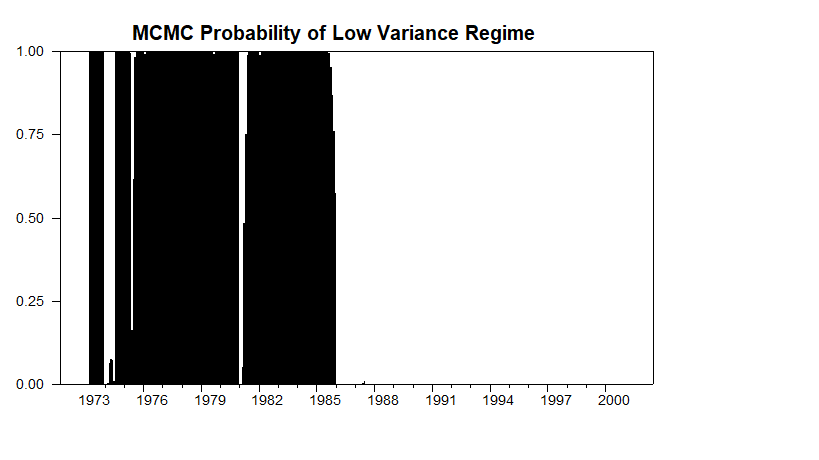
Outside the loop, this computes and graphs the estimated probabilities of the two regimes. Because Gibbs sampling is a "smoothing" procedure, these are the smoothed probabilities.

set regime1 gstart gend = regime1/ndraws

graph(header="MCMC Probability of Low Variance Regime",style=bar)

# regime1

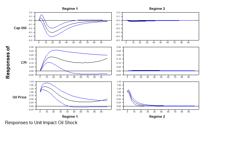
and this graphs the responses to the (standardized) oil shocks.

@MCGraphIRF(model=MSSysRegModel,onlyshocks=||2*oilpos-1,2*oilpos||,$

shocklabels=||"Regime 1","Regime 2"||,$

varlabels=||"Cap Util","CPI","Oil Price"||,$

footer="Responses to Unit Impact Oil Shock")

Graphs

This is the smoothed probability of the regimes calculated using Gibbs sampling. (Fraction of samples where an entry is in regime 1). Note that this is very close to being a permanent sample break rather than a Markov regime switch.

These are the responses of the three variables to the standardized Cholesky factor shocks to the oil price. Because oil price is last in the order, the zero impacts of oil prices on the other two variables is by construction and the unit impact of oil on itself is due to the standardization. Because the data are in 100*log(x), these can all be read as percentages, so in regime 1, a 1% increase in oil prices would produce a .3% maximum drop in capacity utilization about 18 months out. And in regime 2, a 1% increase does effectively nothing to either of the other variables.