EXAMPLEFIVE.RPF

EXAMPLEFIVE.RPF is the example from Section 1.6 in the Introduction. This works with cross section data, showing the use of the SMPL option to restrict subsamples based upon the value of a series, and use of SCATTER to generate an x-y graph.

Full Program

open data wages1.dat
data(format=prn,org=columns) 1 3294 exper male school wage
*
* Do basic statistics on the two subsamples. The first is where "male" is
* non-zero, the second where .not.male is non-zero, that is, where male
* itself is zero.
*
stats(smpl=male) wage
stats(smpl=.not.male) wage
*
* The regression on constant and the male dummy will give the same type
* of information in a form which will usually be easier to interpret. The
* coefficient on the intercept will be the same as the mean for the
* females, while the coefficient on the male dummy is the difference
* between the mean for males and the mean for females.
*
linreg wage
# constant male
*
* Adds school and exper to the regression and test the joint
* significance of the two additional variables.
*
linreg wage
# constant male school exper
*
* This is generated by the Regression Tests Wizard
*
test(zeros)
# 3 4
*
* The same test can also be done using EXCLUDE
*
exclude
# school exper
*
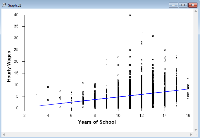
* Generate the fitted values from the original regression and do an
* Actual-Fitted graph.
*
linreg wage
# constant school
prj wagefit
*
scatter(style=symbols,overlay=lines,ovsame,$
vlabel="Hourly Wages",hlabel="Years of School") 2
# school wage
# school wagefit

Output

Statistics on Series WAGE

Observations 1725 Skipped/Missing 1569

Sample Mean 6.313021 Variance 12.242031

Standard Error 3.498861 SE of Sample Mean 0.084243

t-Statistic (Mean=0) 74.938512 Signif Level (Mean=0) 0.000000

Skewness 1.921402 Signif Level (Sk=0) 0.000000

Kurtosis (excess) 8.845542 Signif Level (Ku=0) 0.000000

Jarque-Bera 6685.148147 Signif Level (JB=0) 0.000000

Statistics on Series WAGE

Observations 1569 Skipped/Missing 1725

Sample Mean 5.146924 Variance 8.272740

Standard Error 2.876237 SE of Sample Mean 0.072613

t-Statistic (Mean=0) 70.881766 Signif Level (Mean=0) 0.000000

Skewness 1.977027 Signif Level (Sk=0) 0.000000

Kurtosis (excess) 10.989324 Signif Level (Ku=0) 0.000000

Jarque-Bera 8917.135961 Signif Level (JB=0) 0.000000

Linear Regression - Estimation by Least Squares

Dependent Variable WAGE

Usable Observations 3294

Degrees of Freedom 3292

Centered R^2 0.0317459

R-Bar^2 0.0314517

Uncentered R^2 0.7639932

Mean of Dependent Variable 5.7575850178

Std Error of Dependent Variable 3.2691857840

Standard Error of Estimate 3.2173642756

Sum of Squared Residuals 34076.917047

Regression F(1,3292) 107.9338

Significance Level of F 0.0000000

Log Likelihood -8522.2280

Durbin-Watson Statistic 1.8662

Variable Coeff Std Error T-Stat Signif

************************************************************************************

1. Constant 5.1469238679 0.0812248211 63.36639 0.00000000

2. MALE 1.1660972915 0.1122421588 10.38912 0.00000000

Linear Regression - Estimation by Least Squares

Dependent Variable WAGE

Usable Observations 3294

Degrees of Freedom 3290

Centered R^2 0.1325877

R-Bar^2 0.1317968

Uncentered R^2 0.7885729

Mean of Dependent Variable 5.7575850178

Std Error of Dependent Variable 3.2691857840

Standard Error of Estimate 3.0461431195

Sum of Squared Residuals 30527.870207

Regression F(3,3290) 167.6302

Significance Level of F 0.0000000

Log Likelihood -8341.0906

Durbin-Watson Statistic 1.9051

Variable Coeff Std Error T-Stat Signif

************************************************************************************

1. Constant -3.380018181 0.464976503 -7.26922 0.00000000

2. MALE 1.344368629 0.107675888 12.48533 0.00000000

3. SCHOOL 0.638797702 0.032795844 19.47801 0.00000000

4. EXPER 0.124825450 0.023762761 5.25299 0.00000016

Null Hypothesis : The Following Coefficients Are Zero

SCHOOL

EXPER

F(2,3290)= 191.24105 with Significance Level 0.00000000

Null Hypothesis : The Following Coefficients Are Zero

SCHOOL

EXPER

F(2,3290)= 191.24105 with Significance Level 0.00000000

Linear Regression - Estimation by Least Squares

Dependent Variable WAGE

Usable Observations 3294

Degrees of Freedom 3292

Centered R^2 0.0798020

R-Bar^2 0.0795225

Uncentered R^2 0.7757067

Mean of Dependent Variable 5.7575850178

Std Error of Dependent Variable 3.2691857840

Standard Error of Estimate 3.1365065226

Sum of Squared Residuals 32385.620064

Regression F(1,3292) 285.4910

Significance Level of F 0.0000000

Log Likelihood -8438.3863

Durbin-Watson Statistic 1.8265

Variable Coeff Std Error T-Stat Signif

************************************************************************************

1. Constant -0.722506571 0.387391365 -1.86506 0.06226247

2. SCHOOL 0.557161695 0.032975021 16.89648 0.00000000

Graph