Filardo JBES 1994

Filardo(1994) is the earliest published application in the economics literature of a Markov Switching Model with Time-Varying Transition Probabilities (MS-TVTP). Unfortunately, the results in the paper have a number of clear errors, and can't be reproduced from the data provided by the author. Kim and Nelson(1999) provide an reconstructed data set which we are using.

This is basically the Hamilton(1989) model (HAMILTON.RPF example) with the addition of making the transition probabilities dependent upon a time-varying variable. The particular form of these probabilities is the logistic

$1/\left( {1 + \exp \left( { - \left( {{c_0} + {c_1}{z_t}} \right)} \right)} \right)$

If $c_1$ is zero, this will be a fixed probability. Other papers have used a Normal rather than a logistic, but the logistic is more convenient for EM estimation.

The model is fit to the growth rate of IP with the (lagged) growth of a leading indicator used in calculating the transition probabilities:

set grip = 100.0*log(ip/ip{1})

set glix = 100.0*log(lix/lix{1})

As in the original paper, the dependent variable is rescaled using the relative variances from the earlier part of the sample to the later part. Since rescaling changes the mean, this is not a good idea—there are better ways to adjust the model for exogenous changes in the variance.

stats(noprint) grip * 1959:12

compute stdearly=sqrt(%variance)

stats(noprint) grip 1960:1 *

compute stdlate=sqrt(%variance)

set grip = %if(t<=1959:12,grip*stdlate/stdearly,grip)

This uses @MSVARSetup to set up a mean switching autoregression with 4 lags:

compute nlags=4

compute gstart=1948:7,gend=1991:4

* Standard "Hamilton" model with 4 lags and (only) means switching

@MSVARSetup(lags=nlags,switch=m)

# grip

It first estimates the MS model with fixed transition probabilities (output here):

nonlin(parmset=common) mu phi sigma

nonlin(parmset=fixed) p

frml loglmsvar = log(%MSVarProb(t))

@MSVARInitial gstart gend

maximize(start=(pstar=%MSVARInit()),parmset=fixed+common,$

pmethod=simplex,piters=10,method=bfgs) loglmsvar gstart gend

This sets up the structure for the time-varying transition probabilities—these will be given content later. This allows for the possibility of more than one shift variable in the transition probabilities (as the parameters will be in a VECTOR and the variances in an EQUATION rather and thus can easily be adjusted):

dec equation p1eq p2eq

dec vector v1 v2

nonlin(parmset=tv) v1 v2

You need to create a FUNCTION of the entry which returns either the $M-1 \times M $ or full $M \times M$ transition matrix. Here, we take the logistic of linear functions for the two transitions. %EQNVALUE(eqn,time,v) returns X(time)•v where X is the list of explanatory variables for the equation. Note that this is parameterizing p(1,2) (the transition from 2 to 1) as having positive coefficients. If you want to model directly p(2,2) (which is implicitly 1-p(1,2)), you would just make it %logistic(-%eqnvalue(...

function %MSPTV time

type rect %MSPTV

type integer time

local rect p(1,2)

compute p(1,1)=%logistic(%eqnvalue(p1eq,time,v1),1.0)

compute p(1,2)=%logistic(%eqnvalue(p2eq,time,v2),1.0)

compute %MSPTV=p

end

This registers the FUNCTION for use in the Markov Switching procedures:

@MSPChangeFnc %MSPTV

One special complication of the MS-TVTP model is that there is no obvious initialization for the pre-sample regime probabilities. (With fixed probabilities, there is a stationary calculation available). The choice will typically have a modest effect on the log likelihood for the first few data points and thus will change the estimates somewhat. This uses the stationary solution based upon the transition probabilities computed at the first entry of the sample range. It's a FUNCTION which will be called at the start of each function evaluation.

function TVPInit

type vector TVPInit

compute p=%MSPTV(gstart)

compute TVPInit=%MSVARInit()

end

This finally puts content to the transition probabilities, defining the equations which as used in the linear indexes for the logistics. You can change the explanatory variables to change the probability calculation. This uses the same explanatory variables in each (lag of the growth rate of the leading indicator), though that isn't required. The EQUATION names need to be the ones used in defining the transition probability function above.

equation p1eq *

# constant glix{1}

equation p2eq *

# constant glix{1}

This sets the guess values for the two VECTOR's of coefficients on the logistic indexes. These are .70 and .95 probabilities of remaining in current states (so .05 of switching from 2 to 1), with 0 coefficients on the time-varying coefficient. In this case, the guess values for the other coefficients on the models (the means, variance and autoregressive coefficients) will come from the fixed probability estimation. If you skip that step, you can do @MSVARInitial to get standard guess values.

compute v1=log(.70/(1-.70))*%unitv(%eqnsize(p1eq),1)

compute v2=log(.05/(1-.05))*%unitv(%eqnsize(p2eq),1)

This actually does the maximum likelihood estimation (output here). The PARMSET is the combination of TV (the V1 and V2 that control the time-varying probabilities) plus COMMON (which are the means, variance and autoregressive coefficients that are present both in the fixed and time-varying probability models). The START option computes the initial probabilities of the regimes (in this case, the expanded regimes, since the likelihood depends upon lagged regimes).

maximize(parmset=tv+common,start=(pstar=TVPInit()),$

pmethod=simplex,piters=10,method=bfgs) loglmsvar gstart gend

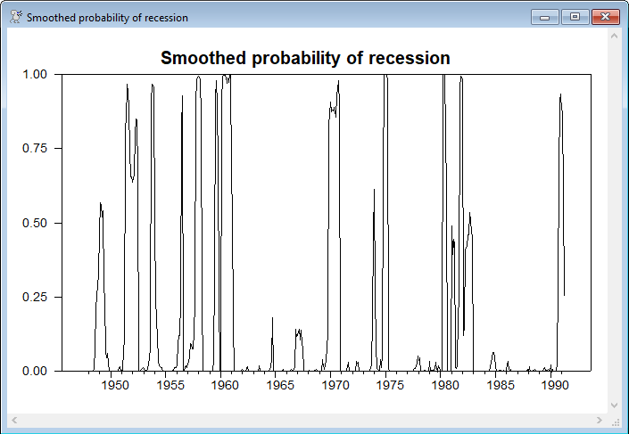
This computes and graphs the smoothed probabilities of the regimes:

@MSVARSmoothed gstart gend psmooth

set precess = psmooth(t)(1)

graph(header="Smoothed probability of recession")

# precess

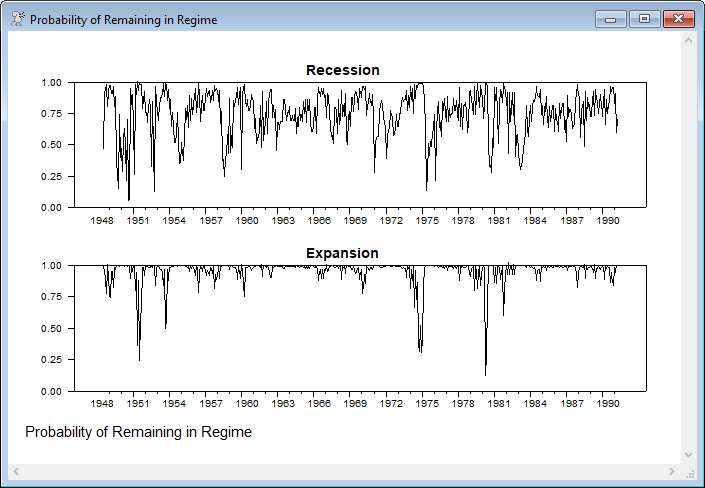
The following computes and graphs the (time-varying) probabilities of remaining in the current regime. With the standard labeling, regime 1 is "recession" and regime 2 is "expansion". The probability of remaining in regime 2 is computed by subtracting 1 from the probability of switching from 2 to 1, since that's what's actually estimated directly.

set p11 gstart gend = %MSPTV(t)(1,1)

set p22 gstart gend = 1.0-%MSPTV(t)(1,2)

spgraph(footer="Probability of Remaining in Regime",vfields=2)

graph(min=0.0,max=1.0,header="Recession")

# p11

graph(min=0.0,max=1.0,header="Expansion")

# p22

spgraph(done)

The remainder of the program estimates the model by EM. This isn't really necessary in this case, since the univariate model has relatively few parameters—the efficiency of EM would be more noticeable if you were doing an actual VAR rather than just an AR. If you want more details about this (which is actually generalized EM, since it takes just one step in a non-linear estimation of the transition parameters rather than fully maximizing each time), you should get the Structural Breaks and Switching Models e-course.

Output

MAXIMIZE - Estimation by BFGS

Convergence in 11 Iterations. Final criterion was 0.0000064 <= 0.0000100

Monthly Data From 1948:07 To 1991:04

Usable Observations 514

Function Value -594.8324

Variable Coeff Std Error T-Stat Signif

************************************************************************************

1. P(1,1) 0.762457348 0.067052275 11.37109 0.00000000

2. P(1,2) 0.028062097 0.009675303 2.90038 0.00372706

3. MU(1)(1) -1.420029541 0.202501224 -7.01245 0.00000000

4. MU(2)(1) 0.439303414 0.085033143 5.16626 0.00000024

5. PHI(1)(1,1) 0.276574088 0.055918737 4.94600 0.00000076

6. PHI(2)(1,1) 0.116794026 0.047709211 2.44804 0.01436360

7. PHI(3)(1,1) 0.142844554 0.044068619 3.24141 0.00118939

8. PHI(4)(1,1) 0.099687308 0.048828250 2.04159 0.04119213

9. SIGMA(1,1) 0.457203216 0.030237557 15.12038 0.00000000

MAXIMIZE - Estimation by BFGS

Convergence in 18 Iterations. Final criterion was 0.0000036 <= 0.0000100

Monthly Data From 1948:07 To 1991:04

Usable Observations 514

Function Value -587.2207

Variable Coeff Std Error T-Stat Signif

************************************************************************************

1. V1(1) 1.393107597 0.516144247 2.69907 0.00695343

2. V1(2) -1.154931785 0.609254986 -1.89565 0.05800687

3. V2(1) -4.372241115 0.736762959 -5.93439 0.00000000

4. V2(2) -1.711197179 0.494071196 -3.46346 0.00053327

5. MU(1)(1) -0.897272689 0.202826097 -4.42385 0.00000970

6. MU(2)(1) 0.485826020 0.076695337 6.33449 0.00000000

7. PHI(1)(1,1) 0.193012912 0.049038415 3.93595 0.00008287

8. PHI(2)(1,1) 0.079311094 0.051333193 1.54503 0.12234009

9. PHI(3)(1,1) 0.111656591 0.053218806 2.09807 0.03589928

10. PHI(4)(1,1) 0.120417957 0.047762535 2.52118 0.01169619

11. SIGMA(1,1) 0.492001954 0.035748088 13.76303 0.00000000

EM iteration 1 Log likelihood -645.49196

EM iteration 2 Log likelihood -593.19867

EM iteration 3 Log likelihood -589.42870

EM iteration 4 Log likelihood -587.97946

EM iteration 5 Log likelihood -587.21487

EM iteration 6 Log likelihood -586.72740

EM iteration 7 Log likelihood -586.41261

EM iteration 8 Log likelihood -586.22424

EM iteration 9 Log likelihood -586.12012

EM iteration 10 Log likelihood -586.06472

EM iteration 11 Log likelihood -586.03475

EM iteration 12 Log likelihood -586.01733

EM iteration 13 Log likelihood -586.00606

EM iteration 14 Log likelihood -585.99790

EM iteration 15 Log likelihood -585.99144

EM iteration 16 Log likelihood -585.98601

EM iteration 17 Log likelihood -585.98129

EM iteration 18 Log likelihood -585.97710

EM iteration 19 Log likelihood -585.97334

EM iteration 20 Log likelihood -585.96995

EM iteration 21 Log likelihood -585.96689

EM iteration 22 Log likelihood -585.96411

EM iteration 23 Log likelihood -585.96158

EM iteration 24 Log likelihood -585.95928

EM iteration 25 Log likelihood -585.95719

EM iteration 26 Log likelihood -585.95528

EM iteration 27 Log likelihood -585.95355

EM iteration 28 Log likelihood -585.95197

EM iteration 29 Log likelihood -585.95053

EM iteration 30 Log likelihood -585.94922

EM iteration 31 Log likelihood -585.94802

EM iteration 32 Log likelihood -585.94693

EM iteration 33 Log likelihood -585.94594

EM iteration 34 Log likelihood -585.94504

EM iteration 35 Log likelihood -585.94421

EM iteration 36 Log likelihood -585.94346

EM iteration 37 Log likelihood -585.94278

EM iteration 38 Log likelihood -585.94215

EM iteration 39 Log likelihood -585.94158

EM iteration 40 Log likelihood -585.94106

EM iteration 41 Log likelihood -585.94059

EM iteration 42 Log likelihood -585.94015

EM iteration 43 Log likelihood -585.93975

EM iteration 44 Log likelihood -585.93939

EM iteration 45 Log likelihood -585.93906

EM iteration 46 Log likelihood -585.93876

EM iteration 47 Log likelihood -585.93848

EM iteration 48 Log likelihood -585.93823

EM iteration 49 Log likelihood -585.93800

EM iteration 50 Log likelihood -585.93778

MAXIMIZE - Estimation by BHHH

NO CONVERGENCE IN 20 ITERATIONS

LAST CRITERION WAS 0.0013962

Monthly Data From 1948:07 To 1991:04

Usable Observations 514

Function Value -587.2207

Variable Coeff Std Error T-Stat Signif

************************************************************************************

1. V1(1) 1.393805669 0.448664111 3.10657 0.00189273

2. V1(2) -1.155607166 0.721271827 -1.60218 0.10911585

3. V2(1) -4.371684739 1.014011467 -4.31128 0.00001623

4. V2(2) -1.712737237 0.737820994 -2.32135 0.02026822

5. MU(1)(1) -0.896016934 0.126230891 -7.09824 0.00000000

6. MU(2)(1) 0.485952331 0.063928915 7.60145 0.00000000

7. PHI(1)(1,1) 0.192844438 0.038797289 4.97056 0.00000067

8. PHI(2)(1,1) 0.079132960 0.054148278 1.46141 0.14390233

9. PHI(3)(1,1) 0.111479390 0.051760318 2.15376 0.03125886

10. PHI(4)(1,1) 0.120290547 0.048477677 2.48136 0.01308823

11. SIGMA(1,1) 0.492021883 0.028998120 16.96737 0.00000000

Graphs

It's important not to over-analyze these results. For instance, the time-varying probability of staying in the recession regime is often quite high, but being near one when the probability of actually being in recession is effectively zero (such as through most of the 1960's) has no real effect on the estimates. The parameters of that govern the 1,1 probability will largely be determined by the relatively small number of entries where the probability of being in recession is fairly high.