For the simple GARCH(1,1) model, the variance evolves according to

\begin{equation} h_t = c + a u_{t - 1}^2 + b h_{t - 1} \end{equation}

The forecast of \(h_{t+k}\) given information at time \(t-1\) (denoted \(\Omega _{t-1}\)) can be derived as

\begin{equation} \begin{split} E\left( {h_{t + k} |\Omega _{t - 1} } \right) &= c +aE\left( {u_{t + k - 1}^2 |\Omega _{t - 1} } \right) + bE\left( {h_{t + k - 1} |\Omega _{t - 1} } \right)\\ &= c + (a + b)E\left( {h_{t + k - 1} |\Omega _{t - 1} } \right) \\ \end{split} \end{equation}

(as long as \(k>0\)) which uses the fact that the expectation of the squared residuals is \(h\) by definition. Thus, multiple step forecasts can be obtained recursively. Note that the coefficient on the lagged term in the forecasting equation is the sum of the coefficients on the lagged variance term and the lagged squared residuals. When \(k=0\), we would be able to use sample values for both \(h_{t - 1} \) and \(u_{t - 1}^2 \).

 

Even though there are parallels in the structure, forecasting an ARCH or GARCH model is more complicated than forecasting an ARMA model, because the out-of-sample “residuals” can’t simply be set to zero, as they enter as squares. The process below does the forecasts by defining two formulas: one produces a recursive estimate of the variance, the other produces the expected value of the squared residuals. Out-of-sample, these are, of course, the same. They differ, however, in their values at the end of the sample, where the lagged UU series are the sample values of the squared residuals, while the lagged HT series are the estimated variances.

 

In GARCHUV.RPF, this estimates a GARCH(1,1) model with an AR(1) mean and forecasts 40 periods out-of-sample. We need both the HSERIES and RESIDS options on the GARCH instruction, since both pieces are needed in constructing the forecasts.

 

linreg(define=ar1) dlogdm

# constant dlogdm{1}

garch(p=1,q=1,equation=ar1,hseries=ht,resids=at)

 

Create the historical UU series

 

set uu = at^2

 

Copy the coefficients out of the %BETA vector. (%NREGMEAN on GARCH is equal to the number of coefficients in the mean model, so this can be used on any GARCH(1,1) regardless of the mean model chosen). The C, A and B will always be in the %BETA vector in that order.

 

compute vc=%beta(%nregmean+1),va=%beta(%nregmean+2),vb=%beta(%nregmean+3)

 

This defines a FRML for extrapolating the variance out-of-sample, and a separate FRML for defining the UU out-of-sample. (Note that the lagged UU is the sample estimate in the first forecast period). The model GARCHMOD combines the two.

 

frml hfrml  ht = vc + vb*ht{1} + va*uu{1}

frml uufrml uu = ht

 

group garchmod hfrml>>ht uufrml>>uu ar1>>meanf

forecast(model=garchmod,from=%regend()+1,steps=40)

 

This forecasts the mean over the same period, and graphs the forecasts of that with +/- 2 GARCH model estimates of the standard deviation.

 

uforecast(equation=ar1,from=%regend()+1,steps=40) modelfore

set upper %regend()+1 %regend()+40 = modelfore+2.0*sqrt(ht(t))

set lower %regend()+1 %regend()+40 = modelfore-2.0*sqrt(ht(t))

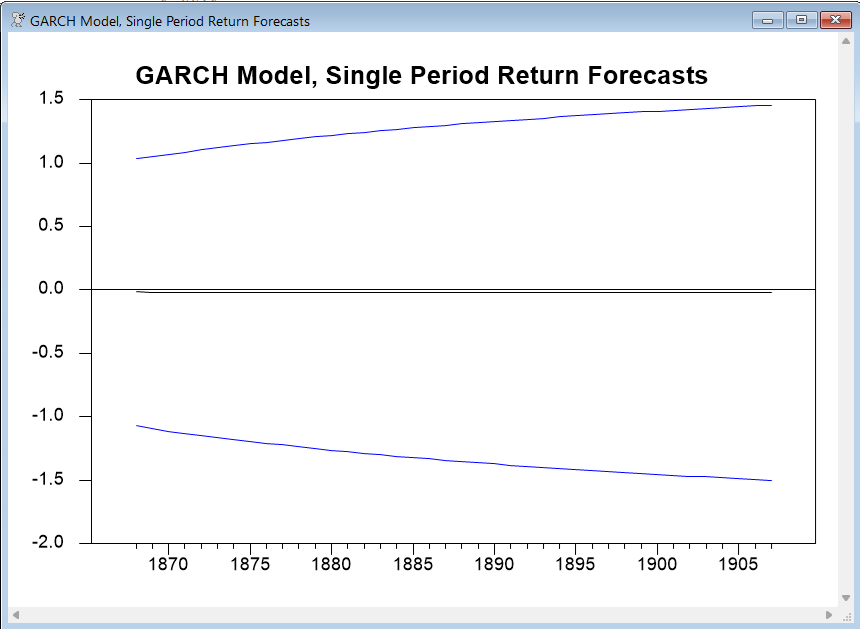
graph(header="GARCH Model, Single Period Return Forecasts") 3

# modelfore

# upper / 2

# lower / 2

VaR Calculations

You might note that the graph of the forecasts is not particularly interesting. It's important to note that what this is computing and graphing are the forecasts of the one period return many steps out, that is, the value at period 1900 is the forecast given data through 1867 of the return from 1899 to 1900. The mean forecast rather quickly converges to the unconditional mean of the process and the forecast of the variance converges (somewhat more slowly) to the unconditional variance.

 

By contrast, a Value at Risk (VaR) calculation is generally based upon the distribution of a holding period return for a certain number of periods. If the data are log period-to-period returns, then the log n-period returns will be the sum of the n consecutive period-to-period returns. The mean forecast of the n-period return will be the sum of the forecast period-to-period returns over n periods (because the mean of the sum is the sum of the mean) and the variance of the n-period return is the sum of the forecast of the period-to-period variance over the n periods because (by assumption) the returns are uncorrelated. Note they are uncorrelated (thus the variance of the sum is the sum of the variance), but not independent because of the dynamics in the variance.

 

The following (again from GARCHUV.RPF) continues the analysis above to compute an approximation to the VaR for the 40 periods forecast. The SSTATS sums the forecast variances (HT series) into the variable VAR40 and the forecast means (MODELFORE series) into the series MEAN40.

 

sstats %regend()+1 %regend()+40 ht>>var40 modelfore>>mean40

 

The Value at Risk is an estimate of the amount that could be lost at chosen tail probability for a given investment. Conventionally, it is cited as a positive number. In this case, given the how the dependent variable is formed, the investment would be a $100 US invested in DM.

 

compute alpha=.01

compute VaR=-mean40-%invnormal(alpha)*sqrt(var40)

?"40 Period VaR at .01" VaR

 

The result is 10.49, so the probability of losing more than 10.49 is 1% using a Normal distribution. Note, however, that the multi-step distribution is not Normal even if the conditional one-step-density is. (In fact, it has no known distribution). To do a calculation which allows for the actual distribution of the multi-step returns requires simulation methods. See, for instance, GARCHBOOT.RPF, which does bootstrapping.

Asymmetry

In the GJR model, the variance evolves according to:

\begin{equation} h_t = c + a u_{t - 1}^2 + b h_{t - 1} + d u_{t - 1}^2 I_{u \le 0} \left( {u_{t - 1} } \right) \end{equation}

For any symmetrical distribution, \(E\left( {u^2 I_{u \le 0} (u)} \right) = (1/2)Eu^2 \) so the forecast for steps beyond the first one will be

\begin{equation} E\left( {h_{t + k} |\Omega _{t - 1} } \right) = c + (a + b + d/2)E\left( {h_{t + k - 1} |\Omega _{t - 1} } \right) \end{equation}

However, note that the first step of forecast has actual data, so the lagged asymmetry term will be either \(u_{t - 1}^2 \) or 0 depending upon the sign of \(u\). The forecast model needs an extra term to take care of this. (The UUS is for UU signed).

 

garch(p=1,q=1,asymmetric,hseries=ht,resids=at) / dlogdm

set uu  = at^2

set uus = at^2*(at<=0)

compute vc=%beta(%nregmean+1),va=%beta(%nregmean+2),vb=%beta(%nregmean+3),vd=%beta(%nregmean+4)

frml hfrml  ht = vc + vb*ht{1} + va*uu{1} + vd*uus{1}

frml uufrml uu = ht

frml uusfrml uus = ht*.5

group agarchmod hfrml>>ht uufrml>>uu uusfrml>>uus

forecast(model=agarchmod,from=%regend()+1,steps=40)

 

EGARCH Models

While this type of recursive calculation works for the simple ARCH and GARCH models, it doesn’t work for an EGARCH model. Forecasts for those have to be done by simulation or bootstrapping. See EGARCHBOOTSTRAP.RPF and EGARCHSIMULATE.RPF as examples.

Forecast Error Analysis

Note that while the above can forecast the mean or variance or both, conventional measures of forecasting performance aren't particularly useful for either. The Root Mean Square Error (RMSE) or Mean Absolute Error (MAE) computed by, for instance, the @UFOREERRORS procedure treat all observations equally—they’re really designed for homoscedastic error processes. Because of this, even if the GARCH process is correct, there is no reason to believe that the mean model estimated with GARCH errors would give better error statistics than simple least squares estimates.

 

These are even less useful for forecasts of the variance as described in "True Volatility is Unobservable". Note, for instance, the result cited from Patton that the MAE is lower for models that systematically underestimate the volatility.

 

Graph

 

Copyright © 2026 Thomas A. Doan