GARCHIMPORT.RPF

GARCHIMPORT.RPF is an example of importance sampling, applied to Monte Carlo integration on a GARCH model.

The log likelihood for a GARCH model has a non-standard form, so it isn’t possible to draw directly from the posterior distribution, even with “flat” priors. Importance sampling is one way to conduct a Bayesian analysis of such a model. An alternative is shown in GARCHGIBBS.RPF.

The importance function used here is a multivariate Student-t, with the mean being the maximum likelihood estimate and the covariance matrix being the estimated covariance matrix from GARCH. This is fattened up by using 5 degrees of freedom. (Note that the GARCH model itself is being estimated assuming Normal residuals. The fat-tailed t is used only for the importance function).

The true density function is computed using GARCH with an input set of coefficients and METHOD=EVAL which does a single function evaluation at the initial guess values. Most instructions which might be used in this way (BOXJENK, CVMODEL, FIND, MAXIMIZE, NLLS) have METHOD=EVAL options.

The example uses a GARCH model on the US 3-month Treasury Bill rate. The “mean model” is a one lag autoregression. This estimates a linear regression to get its residual variance for use as the pre-sample value throughout the analysis.

linreg ftbs3

# constant ftbs3{1}

compute h0=%sigmasq

Estimate a GARCH with Normally distributed errors

garch(p=1,q=1,reg,presample=h0,distrib=normal) / ftbs3

# constant ftbs3{1}

Set up for importance sampling.

FXX is the factor of the covariance matrix of coefficients

XBASE is the estimated coefficient vector

FBASE is the log likelihood (thus the function value at XBASE).

compute fxx =%decomp(%xx)

compute xbase=%beta

compute fbase=%logl

This is the desired number of draws and the degrees of freedom of the multivariate $t$ distribution from which we’re drawing.

compute ndraws=10000

compute drawdf=5.0

Initialize vectors for the first and second moments of the coefficients

compute sumwt=0.0, sumwt2=0.0

compute [vect] b = %zeros(%nreg,1)

compute [symm] bxx = %zeros(%nreg,%nreg)

dec vect u(%nreg) betau(%nreg)

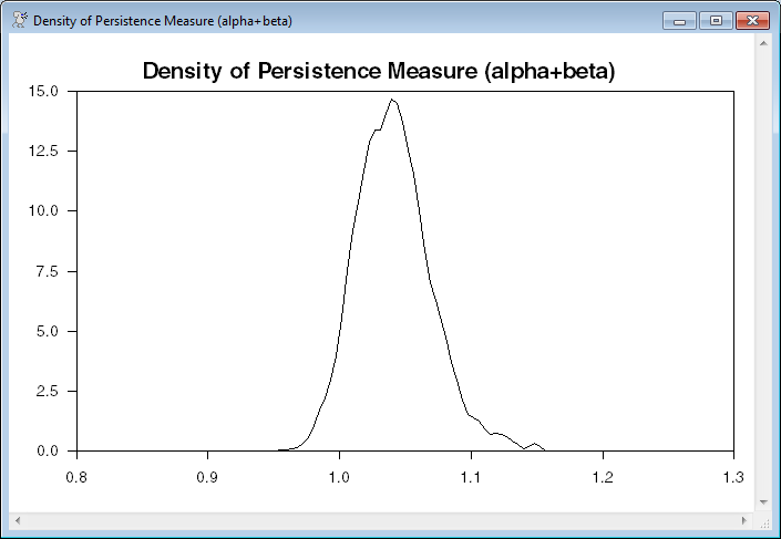
This is used for an estimated density of the persistence measure (ALPHA+BETA). We need to keep the values of the draws and the observation weights in order to use the DENSITY instruction.

set persist 1 ndraws = 0.0

set weights 1 ndraws = 0.0

The pseudo-code for the draw loop is

do draw=1,ndraws

...draw a random set of coefficients from a multivariate t with mean XBASE, scale covariance matrix with factor FXX and DRAWDF degrees of freedom.

...evaluate the GARCH log likelihood and compute the weight

...save the weight on the draw and do whatever other bookeeping is required

end do draw

The random set of coefficients is done easily with the help of the %RANMVT function:

compute betau=xbase+%ranmvt(fxx,drawdf)

As a side effect, %RANMVT fills in the value that can be obtained with %RANLOGKERNEL, which will have the log of the density at the draw relative to the density at the mean (XBASE):

compute gx = %ranlogkernel()

GARCH with EVAL and INIT=BETAU (the drawn set of coefficients) is used to compute the log likelihood:

garch(p=1,q=1,reg,presamp=h0,method=eval,init=betau) / ftbs3

# constant ftbs3{1}

We then need to compute the difference between the log likelihood at the draw and the log likelihood at the mode:

compute fx = %logl-fbase

The one complication is that it is possible for %LOGL to be NA in the GARCH model (if the GARCH parameters go sufficiently explosive). If it is, make the weight zero. Otherwise, exp(...) the difference in the log densities to get the weight.

compute weight = %if(%valid(%logl),exp(fx-gx),0.0)

For the bookkeeping, we are saving the (weighted) sums of the first and second moments of the coefficient vector. We are also saving the full draw history of the persistence measure (which is the sum of the 4th and 5th elements of the BETAU).

compute sumwt = sumwt+weight, sumwt2 = sumwt2+weight^2

compute b = b+weight*betau, bxx = bxx+weight*%outerxx(betau)

compute persist(draw) = betau(4)+betau(5)

compute weights(draw) = weight

Processing the Results

The efficacy of importance sampling depends upon function being estimated, but the following is a simple estimate of the number of effective draws.

?"Effective Sample Size" sumwt^2/sumwt2

Transform the accumulated first and second moments into mean and variance

compute b = b/sumwt, bxx = bxx/sumwt-%outerxx(b)

Create a table with the Monte Carlo means and standard deviations

report(action=define)

report(atrow=1,atcol=1,fillby=cols) "a" "b" "gamma" "alpha" "beta"

report(atrow=1,atcol=2,fillby=cols) b

report(atrow=1,atcol=3,fillby=cols) %sqrt(%xdiag(bxx))

report(action=show)

Estimate the density of the persistence measure and graph it.

density(weights=weights,smpl=weights>0.00,smoothing=1.5) $

persist 1 ndraws xx dx

scatter(style=line,header=$

"Density of Persistence Measure (alpha+beta)")

# xx dx

Full Program

open data haversample.rat

calendar(m) 1957

data(format=rats) 1957:1 2006:12 ftbs3

graph(header="US 3-Month Treasury Bill Rate")

# ftbs3

* Estimate a linear regression to get its residual variance for use as

* the pre-sample value.

linreg ftbs3

# constant ftbs3{1}

compute h0=%sigmasq

* Estimate a GARCH with Normally distributed errors

garch(p=1,q=1,reg,presample=h0,distrib=normal) / ftbs3

# constant ftbs3{1}

compute normallogl=%logl

* Set up for importance sampling.

* FXX is the factor of the covariance matrix of coefficients

* XBASE is the estimated coefficient vector

* FBASE is the final log likelihood

compute fxx =%decomp(%xx)

compute xbase=%beta

compute fbase=%logl

* This is the number of draws and the degrees of freedom of the

* multivariate t distribution from which we're drawing.

compute ndraws=10000

compute drawdf=5.0

* Initialize vectors for the first and second moments of the coefficients

compute sumwt=0.0,sumwt2=0.0

compute [vect] b=%zeros(%nreg,1)

compute [symm] bxx=%zeros(%nreg,%nreg)

dec vect u(%nreg) betau(%nreg)

* This is used for an estimated density of the persistence measure

* (alpha+beta). We need to keep the values of the draws and the

* observation weights in order to use the density instruction.

set persist 1 ndraws = 0.0

set weights 1 ndraws = 0.0

do draw=1,ndraws

* Draw coefficients from a multivariate t

compute betau=xbase+%ranmvt(fxx,drawdf)

* Compute the density of the draw relative to the density at the

* mode. The log of this is returned by the value of %ranlogkernel()

* from the %ranmvt function.

compute gx=%ranlogkernel()

* Compute the log likelihood at the drawn value of the coefficients

garch(p=1,q=1,reg,presample=h0,method=eval,initial=betau) / ftbs3

# constant ftbs3{1}

* Compute the difference between the log likelihood at the draw and

* the log likelihood at the mode.

compute fx=%logl-fbase

* It's quite possible for %logl to be NA in the GARCH model (if the

* GARCH parameters go sufficiently explosive). If it is, make the

* weight zero. Otherwise exp(...) the difference in the log densities.

compute weight=%if(%valid(%logl),exp(fx-gx),0.0)

* Update the accumulators. These are weighted sums.

compute sumwt=sumwt+weight,sumwt2=sumwt2+weight^2

compute b=b+weight*betau

compute bxx=bxx+weight*%outerxx(betau)

* Save the drawn value for persist and weight.

compute persist(draw)=betau(4)+betau(5)

compute weights(draw)=weight

end do draws

* The efficacy of importance sampling depends upon function being

* estimated, but the following is a simple estimate of the number of

* effective draws.

disp "Effective Sample Size" sumwt^2/sumwt2

* Transform the accumulated first and second moments into mean and

* variance.

compute b=b/sumwt,bxx=bxx/sumwt-%outerxx(b)

* Create a table with the Monte Carlo means and standard deviations

report(action=define)

report(atrow=1,atcol=1,fillby=cols) "a" "b" "gamma" "alpha" "beta"

report(atrow=1,atcol=2,fillby=cols) b

report(atrow=1,atcol=3,fillby=cols) %sqrt(%xdiag(bxx))

report(action=show)

* Estimate the density of the persistence measure and graph it

density(weights=weights,smpl=weights>0.00,smoothing=1.5) $

persist 1 ndraws xx dx

scatter(style=line,header=$

"Density of Persistence Measure (alpha+beta)")

# xx dx

Output

Linear Regression - Estimation by Least Squares

Dependent Variable FTBS3

Monthly Data From 1957:02 To 2006:12

Usable Observations 599

Degrees of Freedom 597

Centered R^2 0.9719842

R-Bar^2 0.9719373

Uncentered R^2 0.9941920

Mean of Dependent Variable 5.3828881469

Std Error of Dependent Variable 2.7551056598

Standard Error of Estimate 0.4615335100

Sum of Squared Residuals 127.16886894

Regression F(1,597) 20712.4001

Significance Level of F 0.0000000

Log Likelihood -385.7953

Durbin-Watson Statistic 1.3186

Variable Coeff Std Error T-Stat Signif

************************************************************************************

1. Constant 0.0816496008 0.0413816505 1.97309 0.04894649

2. FTBS3{1} 0.9853633822 0.0068466985 143.91803 0.00000000

GARCH Model - Estimation by BFGS

Convergence in 38 Iterations. Final criterion was 0.0000046 <= 0.0000100

Dependent Variable FTBS3

Monthly Data From 1957:02 To 2006:12

Usable Observations 599

Log Likelihood -61.3428

Variable Coeff Std Error T-Stat Signif

************************************************************************************

1. Constant 0.0631109748 0.0228117343 2.76660 0.00566440

2. FTBS3{1} 0.9900702410 0.0051585759 191.92705 0.00000000

3. C 0.0014556715 0.0005207479 2.79535 0.00518439

4. A 0.3065910350 0.0432686471 7.08576 0.00000000

5. B 0.7300816921 0.0297683170 24.52546 0.00000000

The remainder is based upon random numbers, and so won't match exactly if you run it.

Effective Sample Size 2993.40310

a 0.062580 0.021771

b 0.990223 0.004923

gamma 0.001834 0.000716

alpha 0.327963 0.051931

beta 0.713289 0.035107

Graphs