Hafner Herwartz JIMF 2006 |
This is a replication file for the analysis in Hafner and Herwartz(2006) (HH for short). The data set is a reproduction, so the results are similar but don't quite match.
This paper defines the concept of a Volatility Impulse Reponse Function or VIRF, which is the response of the variance/covariance matrix to some form of shock. Note that this has very different behavior from a standard Impulse Response Function in a VAR or VECM, which shows the response to the process mean (not variance) to a shock. In standard IRF calculations, the mean of a residual is zero, so anything non-zero is a "shock". In a VIRF for a GARCH model, the residuals have an covariance matrix which is non-zero—not only non-zero, but time-varying. If the variance of component 1 is 4.0, then a residual of 1.0 is not a "shock", but exactly the opposite—it's of a size smaller than expected. Also, unlike standard IRF's, the VIRF's aren't linear in the shock size (doubling the size of a shock doesn't double the response of the variance), so there is no real point to any sort of standardized calculation. Because of this, HH look at historical episodes—it gives you the baseline covariance matrix from the GARCH model and an observable shock that exceeds that.
Note that the VIRF as defined by HH only exists for certain types of models—those that are special cases of the "VECH" model, and only with no asymmetry. This includes BEKK and DVECH, but excludes (for instance) CC and DCC. The excluded models have variances which are more dependent upon initial conditions than is allowed by the VIRF calculation.
This paper and VIRF's in general are covered in greater detail as part of the ARCH, GARCH and Volatility Models e-course.
This describes the program named garchmodels.rpf, which uses some features added with version 10 for better handling daily data with irregular dates (due to holidays). The garchmodels_v9.rpf program (which will work with version 9 and earlier) does the same calculations, but the handling of calendar dates is much clumsier.
The dates on the file are coded into a series called date, which has the date as a six digit number in the form yymmdd. This reads the data, using the %JULIANFROMCODED function to remap the date to its "Julian" value, and sets the CALENDAR based upon that.
open data xrates.xls
data(format=xls,org=columns) 1 3720 usxjpn usxfra usxsui usxnld usxuk $
usxbel usxger usxswe usxcan usxita date
set jdate = %julianfromcoded(date,"yymmdd")
cal(julian=jdate)
This converts the raw exchange rates in the data set to returns (for Germany (DEMRET) and the UK pound (GBPRET) vs the US dollar). This is the transformation used in the paper, but in practice we would recommend multiplying these by 100 to give the data and the variances a more reasonable scale. (In the paper, they have to multiply variances by \(10^4\) to get a reasonable scale on graphs, which is what scaling the data by 100 accomplishes directly).
set demret = log(usxger/usxger{1})
set gbpret = log(usxuk/usxuk{1})
This next fits univariate GARCH models to the two series with univariate AR(1) models for the mean and does some diagnostics on the standardized residuals: a test for residual ARCH, a Jarque-Bera test for Gaussianity, and Q tests for serial correlation. REPORT is used to insert the diagnostics into a single combined table which could be put into a paper.
garch(regressors,robust,hseries=h) / demret
# constant demret{1}
set stdu = %resids/sqrt(h)
report(action=define,title="Table 1: Diagnostic Tests for Univariate Processes")
report(atrow=1,atcol=1,align=center) "ARCH-LM(1)" "JB" "Q(10)" "Q(20)"
report(atrow=2,atcol=1,span) "DEM/USD"
@archtest(noprint,lags=1) stdu
report(atrow=3,atcol=1) %cdstat
report(atrow=4,atcol=1,special=parens) %signif
stats(noprint) stdu
report(atrow=3,atcol=2) %jbstat
report(atrow=4,atcol=2,special=parens) %jbsignif
corr(noprint,number=10,qstats,dfc=1) stdu
report(atrow=3,atcol=3) %qstat
report(atrow=4,atcol=3,special=parens) %qsignif
corr(noprint,number=20,qstats,dfc=1) stdu
report(atrow=3,atcol=4) %qstat
report(atrow=4,atcol=4,special=parens) %qsignif
garch(regressors,robust,hseries=h) / gbpret
# constant gbpret{1}
set stdu = %resids/sqrt(h)
report(atrow=5,atcol=1,span) "GBP/USD"
@archtest(noprint,lags=1) stdu
report(atrow=6,atcol=1) %cdstat
report(atrow=7,atcol=1,special=parens) %signif
stats(noprint) stdu
report(atrow=6,atcol=2) %jbstat
report(atrow=7,atcol=2,special=parens) %jbsignif
corr(noprint,number=10,qstats,dfc=1) stdu
report(atrow=6,atcol=3) %qstat
report(atrow=7,atcol=3,special=parens) %qsignif
corr(noprint,number=20,qstats,dfc=1) stdu
report(atrow=6,atcol=4) %qstat
report(atrow=7,atcol=4,special=parens) %qsignif
report(action=format,atrow=2,picture="*.###",align=decimal)
report(action=show)
The GARCH estimates are fairly typical of daily returns series—for both series, the GARCH persistence (sum of A and B) is just below 1, with most of it coming from the "GARCH" coefficient (B). The AR(1) coefficients in the mean are small, but probably not negligible for the GBPRET estimates. The diagnostics are not unreasonable—the residual ARCH test passes easily; the Q test fails slightly at the .05 level for the German data, but that's not a major problem with such a large data set (over 3000 observations). The JB test for Gaussianity very strongly rejects, but the GARCH model doesn't require normally distributed residuals, so that isn't surprising.
Note that if the intent is to estimate a multivariate GARCH model (as it is here), the univariate models and diagnostics don't help that much—while the AR(1) univariate models seem to be adequate for a univariate model, that doesn't tell you that they are adequate for a bivariate model, since there is no test for cross-series effects. A VAR(1) model is probably a more reasonable choice for the mean if there appears to be some serial correlation in the returns.
That being said, the paper uses a model with separate univariate AR(1) models rather than a full VAR(1) for the bivariate mean model. That's set up and estimated with:
equation demeqn demret
# constant demret{1}
equation gbpeqn gbpret
# constant gbpret{1}
group uniar1 demeqn gbpeqn
garch(model=uniar1,mv=bekk,rvectors=rv,hmatrices=hh,$
stdresids=stdmvu,factorby=eigen)
The GARCH estimates include jointly standardized residuals using an eigen factorization of the covariance matrices. The (non-standardized) residuals are saved using the RVECTORS option as they will be needed for computing the shocks at the historical episodes.
The coefficient estimates for a BEKK model are usually difficult to interpret. HH convert the BEKK estimates to their equivalent VECH form, which tells you more about the dynamics of the variance/covariance matrices, and compute the eigenvalues of the recursion. @MVGARCHtoVECH is a procedure which takes the GARCH output (for certain types of models) and produces the A and B matrices in the implied VECH form.
@MVGARCHtoVECH(mv=bekk)
eigen(cvalues=cv) %%vech_a+%%vech_b
disp "Eigenvalues from BEKK-Gaussian" cv
The largest eigenvalue is 0.98557, that is, just inside the unit circle, so the variance recursion will be fairly persistent, but isn't explosive.
HH then do a multivariate Jarque-Bera test for Gaussianity in the (jointly standardized) residuals—in RATS, this is done with the @MVJB procedure:
@mvjb(sigma=%identity(%nvar))
# stdmvu
which, not surprisingly given the univariate results, overwhelmingly rejects. The estimation of the BEKK model is re-done using t distributed errors, and that is what is used for the remainder of the paper. (Note that the repeat of the multivariate J-B test is not expected to give an acceptance—in fact, you would expect to see an even stronger rejection, as the use of t errors rather than Gaussian errors doesn't penalize outliers as strongly).
garch(model=uniar1,mv=bekk,rvectors=rv,hmatrices=hh,distrib=t,$
stdresids=stdmvu,factorby=eigen)
@MVGARCHtoVECH(mv=bekk)
eigen(cvalues=cv) %%vech_a+%%vech_b
disp "Eigenvalues from BEKK-t" cv
@mvjb(sigma=%identity(%nvar))
# stdmvu
Calculation of VIRF
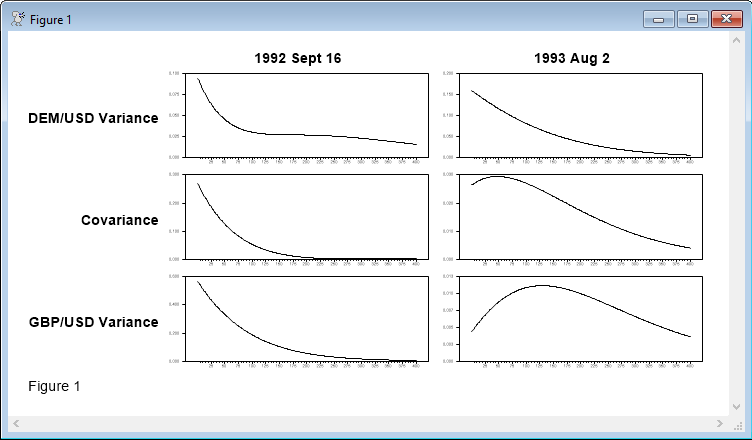
HH compute the VIRF from two episodes in the data. The first is "Black Wednesday'' (September 16, 1992), when the Italian lira and the UK dropped out of the European Exchange Rate Mechanism (ERM). The second is August 2, 1993, when the EC finance ministers changed the variability bands on currencies in the ERM. Responses for 400 steps (roughly 1 1/2 years with five day a week data) are computed.
compute blackwed=1992:09:16
compute ecpolicy=1993:08:02
We'll look at the calculation of the VIRF for the Black Wednesday shock in detail.
compute eps0=rv(blackwed)
compute sigma0=hh(blackwed)
compute shock=1.e+4*%vec(%outerxx(eps0)-sigma0)
EPS0 is the vector of residuals on the date, and SIGMA0 is the model's predicted covariance matrix for that date (that is, the prediction of the variance given data through the day before). The "shock" to the covariance matrix is the difference between the outer product of EPS0 and SIGMA0. (This is multiplied by 10000 to get a better scale for the graphs. As noted above, that wouldn't be necessary if the returns had been scaled up by 100 at the beginning). There are three components to the VECH of 2 by 2 matrix: the (1,1), (2,1) and (2,2) elements of the covariance matrix in that order. This computes and saves the VIRF.
dec vect[series] sept92virf(3)
do i=1,3
set sept92virf(i) 1 nstep = 0.0
end do i
do step=1,nstep
if step==1
compute hvec=%%vech_a*shock
else
compute hvec=(%%vech_a+%%vech_b)*hvec
compute %pt(sept92virf,step,hvec)
end do step
The response for the first step out (for the day after the shock) requires just the "A" term in the VECH representation times the shock, while all remaining ones use both the "A" and "B" terms times the previous step's response. The %PT function unpacks the vector of responses into the separate elements of the time series of responses.
This graphs the responses. Note that this was all enclosed within an SPGRAPH instruction to organize the graphs from the two experiments onto a single page.
do i=1,3
graph(min=0.0,column=1,row=i,picture="*.###",vticks=5,nodates)
# sept92virf(i) 1 nstep
end do i
The EC policy VIRF is done using a "baseline" for the covariance matrix of zero, rather than of the predicted covariance matrix, which is an alternative that they propose. Note that the only difference is that the "shock" calculation doesn't subtract off SIGMA0:
compute eps0=rv(ecpolicy)
compute sigma0=hh(ecpolicy)
compute shock=1.e+4*%vec(%outerxx(eps0))
As would be expected given the near-unit eigenvalues, the effect of a shock (either one) take quite a while to dissipate.
Output
GARCH Model - Estimation by BFGS
Convergence in 18 Iterations. Final criterion was 0.0000011 <= 0.0000100
With Heteroscedasticity/Misspecification Adjusted Standard Errors
Dependent Variable DEMRET
Irregular Data From 1980:01:02 To 1994:04:01
Usable Observations 3718
Log Likelihood 13312.5266
Variable Coeff Std Error T-Stat Signif
************************************************************************************
1. Constant -4.2686e-05 1.3146e-04 -0.32470 0.74540440
2. DEMRET{1} 0.0292 0.0161 1.81967 0.06880870
3. C 1.3640e-06 3.2080e-07 4.25170 0.00002122
4. A 0.0735 9.5631e-03 7.69044 0.00000000
5. B 0.9008 0.0115 78.55691 0.00000000
GARCH Model - Estimation by BFGS
Convergence in 24 Iterations. Final criterion was 0.0000043 <= 0.0000100
With Heteroscedasticity/Misspecification Adjusted Standard Errors
Dependent Variable GBPRET
Irregular Data From 1980:01:02 To 1994:04:01
Usable Observations 3718
Log Likelihood 13356.3494
Variable Coeff Std Error T-Stat Signif
************************************************************************************
1. Constant -6.1799e-05 1.2989e-04 -0.47577 0.63423843
2. GBPRET{1} 0.0564 0.0167 3.36932 0.00075355
3. C 6.5797e-07 2.1892e-07 3.00555 0.00265100
4. A 0.0474 8.2642e-03 5.73904 0.00000001
5. B 0.9395 0.0109 86.48694 0.00000000
DEM/USD
1.103 259.544 19.367 32.157
(0.294) (0.000) (0.022) (0.030)
GBP/USD
0.692 435.111 9.994 24.910
(0.406) (0.000) (0.351) (0.164)
MV-GARCH, BEKK - Estimation by BFGS
Convergence in 53 Iterations. Final criterion was 0.0000074 <= 0.0000100
Irregular Data From 1980:01:02 To 1994:04:01
Usable Observations 3718
Log Likelihood 28606.7936
Variable Coeff Std Error T-Stat Signif
************************************************************************************
Mean Model(DEMRET)
1. Constant -0.000044869 0.000098167 -0.45707 0.64762151
2. DEMRET{1} 0.026382217 0.014787080 1.78414 0.07440096
Mean Model(GBPRET)
3. Constant -0.000059095 0.000093973 -0.62885 0.52944481
4. GBPRET{1} 0.044781074 0.015372533 2.91306 0.00357909
5. C(1,1) 0.000966444 0.000083838 11.52750 0.00000000
6. C(2,1) 0.000450386 0.000125609 3.58562 0.00033628
7. C(2,2) 0.000650053 0.000059989 10.83621 0.00000000
8. A(1,1) 0.287528737 0.019078038 15.07119 0.00000000
9. A(1,2) -0.030077557 0.017118946 -1.75697 0.07892210
10. A(2,1) -0.063615022 0.020189978 -3.15082 0.00162812
11. A(2,2) 0.258475962 0.018273313 14.14500 0.00000000
12. B(1,1) 0.948639022 0.006275196 151.17280 0.00000000
13. B(1,2) 0.016075586 0.005015470 3.20520 0.00134968
14. B(2,1) 0.016759873 0.006616611 2.53300 0.01130910
15. B(2,2) 0.953470924 0.005582240 170.80437 0.00000000
Eigenvalues from BEKK-Gaussian ( 0.98557, 0.00000) ( 0.97697, -0.00679) ( 0.97697, 0.00679)
Var JB P-Value
1 266.040 0.000
2 3292.914 0.000
All 3558.954 0.000
MV-GARCH, BEKK - Estimation by BFGS
Convergence in 74 Iterations. Final criterion was 0.0000000 <= 0.0000100
Irregular Data From 1980:01:02 To 1994:04:01
Usable Observations 3718
Log Likelihood 28984.5373
Variable Coeff Std Error T-Stat Signif
************************************************************************************
Mean Model(DEMRET)
1. Constant -0.000086045 0.000076731 -1.12138 0.26212556
2. DEMRET{1} 0.003503778 0.011771167 0.29766 0.76596445
Mean Model(GBPRET)
3. Constant 0.000029887 0.000073638 0.40587 0.68483983
4. GBPRET{1} 0.018359843 0.011720040 1.56653 0.11722361
5. C(1,1) 0.000962449 0.000122075 7.88409 0.00000000
6. C(2,1) 0.000707654 0.000137086 5.16212 0.00000024
7. C(2,2) -0.000455501 0.000072080 -6.31935 0.00000000
8. A(1,1) 0.289112748 0.024142352 11.97533 0.00000000
9. A(1,2) -0.007043956 0.027323490 -0.25780 0.79656240
10. A(2,1) -0.051853003 0.023502632 -2.20626 0.02736554
11. A(2,2) 0.245709343 0.027364231 8.97922 0.00000000
12. B(1,1) 0.956476832 0.007047515 135.71832 0.00000000
13. B(1,2) 0.004568053 0.008632405 0.52918 0.59668404
14. B(2,1) 0.009988195 0.007467217 1.33761 0.18102485
15. B(2,2) 0.963674467 0.008396694 114.76833 0.00000000
16. Shape(t degrees) 4.386659383 0.245154125 17.89348 0.00000000
Eigenvalues from BEKK-t ( 0.99416, -0.00000) ( 0.99325, 0.00447) ( 0.99325, -0.00447)
Var JB P-Value
1 266.475 0.000
2 5099.162 0.000
All 5365.637 0.000
Copyright © 2026 Thomas A. Doan