MONTEEXOGVAR.RPF

MONTEEXOGVAR.RPF is an example of Monte Carlo integration with shock to an "exogenous" variable. The three variables in the VAR are (log) real GDP, investment and consumption. The exogenous variable is the 3 month T-Bill rate, which is included in the VAR in both current and lagged form.

The shock to the exogenous variable is accomplished by adding a placeholder (basically empty) equation to make it easy to input a unit shock to T-Bills:

equation(empty) rateeq ftb3

The unit shock to the variable is then imposed by using the SHOCKS option applied to the MODEL formed by "adding" the placeholder equation to the VAR-X model.

impulse(noprint,model=varmodel+rateeq,shocks=%unitv(%nvar+1,%nvar+1),$

flatten=%%responses(draw),steps=nstep)

Note that the combined model will have no dynamics for the exogenous variable, so a unit shock will be a +1 at impact followed by zero for the remaining periods. Whether this is reasonable will depend upon the situation. However, it does make the process of drawing coefficients simple because (conditional on the exogenous variable) this is a system of identical equations. An alternative approach for an exogenous variable like this is to do a "near-VAR" where the exogenous variable is included in a separate equation with the other endogenous variables excluded. Monte Carlo integration for such a system is more complicated as it requires Gibbs sampling (see the MONTESUR.RPF and MONTENEARSVAR.RPF examples).

Full Program

compute lags=4        ;*Number of lags
compute nstep=16      ;*Number of response steps
compute ndraws=10000 ;*Number of keeper draws
*
open data haversample.rat
cal(q) 1959
data(format=rats) 1959:1 2006:4 ftb3 gdph ih cbhm
*
* These are transformed to 100*log(x) so responses can be interpreted as
* percentage changes (at annual rate, since the data are in annual
* rates).
*
set loggdp = 100.0*log(gdph)
set loginv = 100.0*log(ih)
set logc   = 100.0*log(cbhm)
*
* T-Bill rate is treated as exogenous, with current and lagged values
* included in the VAR equation.
*
system(model=varmodel)
variables loggdp loginv logc
lags 1 to lags
det constant ftb3{0 to lags}
end(system)
*
* Define placeholder equation to allow shock to T-bills. Note that the
* combined model will have no dynamics for the exogenous variable, so a
* unit shock will be a +1 at impact followed by zero for the remaining
* periods.
*
equation(empty) rateeq ftb3
*
******************************************************************
estimate
compute nshocks=1
compute nvar   =%nvar
compute fxx    =%decomp(%xx)
compute fwish =%decomp(inv(%nobs*%sigma))
compute wishdof=%nobs-%nreg
compute betaols=%modelgetcoeffs(varmodel)
*
declare vect[rect] %%responses(ndraws)
*
infobox(action=define,progress,lower=1,upper=ndraws) "Monte Carlo Integration"
do draw=1,ndraws
   *
   * On the odd values for <<draw>>, a draw is made from the inverse Wishart
   * distribution for the covariance matrix. This assumes use of the
   * Jeffrey's prior |S|^-(n+1)/2 where n is the number of equations in
   * the VAR. The posterior for S with that prior is inverse Wishart with
   * T-p d.f. (p = number of explanatory variables per equation) and
   * covariance matrix inv(T(S-hat)).
   *
   * Given the draw for S, a draw is made for the coefficients by adding
   * the mean from the least squares estimate to a draw from a
   * multivariate Normal with (factor of) covariance matrix as the
   * Kroneker product of the factor of the draw for S and a factor of
   * the X'X^-1 from OLS.
   *
   * On even draws, the S is kept at the previous value, and the
   * coefficient draw is reflected through the mean.
   *
   if %clock(draw,2)==1 {
      compute sigmad =%ranwisharti(fwish,wishdof)
      compute fsigma =%decomp(sigmad)
      compute betau   =%ranmvkron(fsigma,fxx)
      compute betadraw=betaols+betau
   }
   else
      compute betadraw=betaols-betau
   *
   * Push the draw for the coefficient back into the model.
   *
   compute %modelsetcoeffs(varmodel,betadraw)
   *
   * Shock the combination of the VAR + the placeholder equation with a
   * unit shock to the placeholder. Save into %%responses(draw)
   *
   impulse(noprint,model=varmodel+rateeq,shocks=%unitv(%nvar+1,%nvar+1),$
     flatten=%%responses(draw),steps=nstep)
   infobox(current=draw)
end do draw
infobox(action=remove)
*
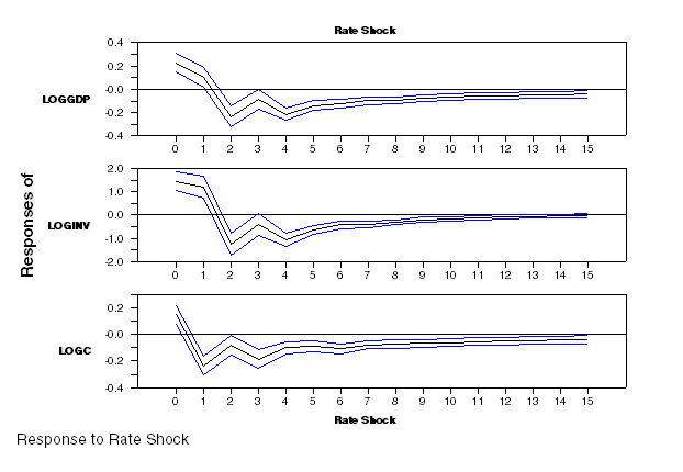
@mcgraphirf(model=varmodel,footer="Response to Rate Shock",$
   shocklabels=||"Rate Shock"||)

Output

VAR/System - Estimation by Least Squares

Quarterly Data From 1960:01 To 2006:04

Usable Observations 188

Dependent Variable LOGGDP

Mean of Dependent Variable 863.24850619

Std Error of Dependent Variable 43.16368147

Standard Error of Estimate 0.71298029

Sum of Squared Residuals 86.417951673

Durbin-Watson Statistic 1.9410

Variable Coeff Std Error T-Stat Signif

************************************************************************************

1. LOGGDP{1} 0.718838723 0.176123342 4.08145 0.00006873

2. LOGGDP{2} 0.163357335 0.250347494 0.65252 0.51494563

3. LOGGDP{3} -0.049907233 0.249392082 -0.20012 0.84162940

4. LOGGDP{4} 0.107198203 0.178582766 0.60027 0.54912445

5. LOGINV{1} 0.009389066 0.028422160 0.33034 0.74154743

6. LOGINV{2} -0.018080246 0.040392920 -0.44761 0.65500505

7. LOGINV{3} 0.001728941 0.039655313 0.04360 0.96527503

8. LOGINV{4} -0.009330677 0.026688422 -0.34962 0.72706024

9. LOGC{1} 0.520033143 0.138831878 3.74578 0.00024599

10. LOGC{2} -0.107711202 0.210256009 -0.51229 0.60911580

11. LOGC{3} -0.187435249 0.212811185 -0.88076 0.37969204

12. LOGC{4} -0.150875564 0.148300659 -1.01736 0.31042660

13. Constant 2.614725395 6.208340823 0.42116 0.67416783

14. FTB3 0.226057456 0.080082307 2.82281 0.00532863

15. FTB3{1} -0.147596514 0.129173735 -1.14262 0.25480300

16. FTB3{2} -0.194607289 0.134893951 -1.44267 0.15095375

17. FTB3{3} 0.156601403 0.137878594 1.13579 0.25764231

18. FTB3{4} -0.075222770 0.090665245 -0.82968 0.40788556

F-Tests, Dependent Variable LOGGDP

Variable F-Statistic Signif

*******************************************************

LOGGDP 100.4703 0.0000000

LOGINV 1.2772 0.2809132

LOGC 6.3103 0.0000930

Dependent Variable LOGINV

Mean of Dependent Variable 661.46375119

Std Error of Dependent Variable 55.77696411

Standard Error of Estimate 3.51221149

Sum of Squared Residuals 2097.0570181

Durbin-Watson Statistic 1.9166

Variable Coeff Std Error T-Stat Signif

************************************************************************************

1. LOGGDP{1} -1.73063638 0.86760102 -1.99474 0.04766955

2. LOGGDP{2} 1.07373460 1.23323654 0.87066 0.38516547

3. LOGGDP{3} 0.22595133 1.22853008 0.18392 0.85429536

4. LOGGDP{4} 0.21639107 0.87971638 0.24598 0.80599583

5. LOGINV{1} 0.96236100 0.14001037 6.87350 0.00000000

6. LOGINV{2} -0.09158183 0.19897952 -0.46026 0.64591953

7. LOGINV{3} -0.01173374 0.19534600 -0.06007 0.95217325

8. LOGINV{4} -0.03916221 0.13146981 -0.29788 0.76615861

9. LOGC{1} 3.75229630 0.68389958 5.48662 0.00000015

10. LOGC{2} -1.87275684 1.03574192 -1.80813 0.07235360

11. LOGC{3} -1.37757956 1.04832897 -1.31407 0.19059242

12. LOGC{4} -0.08781481 0.73054373 -0.12020 0.90446292

13. Constant -37.45332117 30.58290150 -1.22465 0.22240176

14. FTB3 1.44290543 0.39449337 3.65762 0.00033924

15. FTB3{1} -0.31531114 0.63632261 -0.49552 0.62087242

16. FTB3{2} -1.21307881 0.66450096 -1.82555 0.06967307

17. FTB3{3} 0.44073517 0.67920360 0.64890 0.51727871

18. FTB3{4} -0.44173524 0.44662597 -0.98905 0.32404450

F-Tests, Dependent Variable LOGINV

Variable F-Statistic Signif

*******************************************************

LOGGDP 1.2442 0.2941321

LOGINV 102.6901 0.0000000

LOGC 9.7850 0.0000004

Dependent Variable LOGC

Mean of Dependent Variable 822.34192751

Std Error of Dependent Variable 46.40524913

Standard Error of Estimate 0.59669533

Sum of Squared Residuals 60.527704367

Durbin-Watson Statistic 2.0183

Variable Coeff Std Error T-Stat Signif

************************************************************************************

1. LOGGDP{1} -0.097281390 0.147398151 -0.65999 0.51015307

2. LOGGDP{2} 0.115522736 0.209516565 0.55138 0.58209885

3. LOGGDP{3} -0.212689164 0.208716978 -1.01903 0.30963606

4. LOGGDP{4} 0.212090137 0.149456450 1.41908 0.15770760

5. LOGINV{1} 0.036881730 0.023786591 1.55053 0.12287494

6. LOGINV{2} -0.024740586 0.033804955 -0.73186 0.46526007

7. LOGINV{3} 0.030646020 0.033187650 0.92342 0.35709905

8. LOGINV{4} -0.039489328 0.022335620 -1.76800 0.07885504

9. LOGC{1} 1.073911672 0.116188813 9.24281 0.00000000

10. LOGC{2} 0.001888856 0.175963882 0.01073 0.99144799

11. LOGC{3} 0.194241246 0.178102316 1.09062 0.27698527

12. LOGC{4} -0.292144924 0.124113265 -2.35386 0.01972241

13. Constant 1.557053556 5.195778971 0.29968 0.76478991

14. FTB3 0.144393931 0.067021122 2.15445 0.03261232

15. FTB3{1} -0.420582822 0.108105885 -3.89047 0.00014338

16. FTB3{2} 0.141862767 0.112893150 1.25661 0.21061849

17. FTB3{3} -0.075860533 0.115391007 -0.65742 0.51179904

18. FTB3{4} 0.181942232 0.075878014 2.39783 0.01757608

F-Tests, Dependent Variable LOGC

Variable F-Statistic Signif

*******************************************************

LOGGDP 0.6524 0.6259534

LOGINV 1.5581 0.1877602

LOGC 220.6688 0.0000000

Graph

Note that this is intended as an example of the technique rather than as a serious piece of empirical work.

The impact responses appear to be of unexpected sign. (The dependent variables are all in 100*log(x) form so their responses would be interpreted as percentage changes). The C impact is relatively small (roughly 0.1%), but investment is +1.5% (at annual rate) with a fairly tight 16-84% interval. Two possible explanations for this are (a) that T-bills really aren't exogenous (which isn't tested in this) so the interest rate might respond within the quarter to higher than expected investment numbers or (b) that a model with three real variables plus nominal interest rates might not be rich enough to get the dynamics correct, that a price index is necessary as well.