MONTENEARSVAR.RPF

MONTENEARSVAR.RPF is an example of a MCMC (Markov Chain Monte Carlo) analysis of a combination of a near VAR for the lag coefficients and a structural VAR for the covariance matrix. This is based upon the SIMSIRF.RPF example from the Sims and Zha(1999) replication files. However, this is only for illustration—it treats as exogenous a variable which really isn't, which produces some odd results.

Technically, this uses Metropolis-within-Gibbs. The structural (contemporaneous) model is drawn using Random Walk Metropolis. Given the values of the structural parameters, the variances of the shocks can be drawn directly, and given the covariance matrix, the coefficients can be drawn using the standard methods for linear SUR systems of modest size. This uses the @SURGibbsSetup procedures to handle the specialized calculations for Gibbs sampling on the near-VAR.

This same basic method can be used for an informative prior on the lag coefficients combined with a structural model for the covariance matrix. The subcalculation

compute bdraw=%ranmvposthb(hdata,hbdata)

can be replaced by

compute bdraw=%ranmvposthb(hdata+hprior,hbdata+hprior*bprior)

where HPRIOR is the precision matrix on the lag coefficients and BPRIOR is the mean.

Note that this is a very complicated sampling process which may require significant experimentation to achieve reasonable results. If you are unfamiliar with general MCMC sampling, we would recommend the RATS Bayesian Econometrics e-course. The distribution for the random walk increments for the structural models is a multivariate t governed by the following:

* This is the covariance matrix for the RW increment. We might have to

* change the scaling on this to achieve a reasonable acceptance

* probability.

compute f=%decomp(%xx)*.35

compute nudraw=6

Both the scaling (the .35) and the degrees of freedom (the NUDRAW value) may need to be changed in another application to get a reasonable rate of acceptance.

This combines the features of MONTESUR.RPF, which does Gibbs sampling for a "near-VAR", but for a simple contemporaneous model, and MONTESVAR.RPF, which does sampling for a structural contemporaneous model (SVAR) but for a full (OLS) VAR for the lag coefficients.

Full Program

open data simszha.xls
calendar(q) 1948
data(format=xls,org=columns) 1948:01 1989:03 gin82 gnp82 gnp gd lhur fygn3 m1
*
set gin82 = log(gin82)
set gnp82 = log(gnp82)
set gd    = log(gd)
set m1    = log(m1)
set fygn3 = fygn3*.01
set lhur = lhur*.01
*
compute nlags =4
compute nvar =6
compute nsteps=25
compute nburn =2000
compute ndraws=10000
*
* Create a near-VAR that treats gin82 as exogenous.
*
system(model=fivevar)
variables fygn3 m1 gnp82 gd lhur
lags 1 to nlags
det constant gin82{1 to nlags}
end(system)
*
equation gineqn gin82
# constant gin82{1 to nlags}
*
system(model=nearvar)
variables fygn3 m1 gnp82 gd lhur gin82
lags 1 to nlags
det constant
end(system)

*compute nearvar=fivevar+gineqn
*
* Set up the Gibbs sampler for the SUR system
*
@SURGibbsSetup nearvar
*
* Do a SUR to get a set of estimates to initialize the Gibbs sampler.
*
sur(model=nearvar,cvout=sigmaAtBeta)
compute tnobs =%nobs
*
* Create the set of non-linear parameters, and the "A" formula for
* CVMODEL. Since these are all off-diagonal, we can try just zeros
* for the guess values.
*
nonlin(parmset=simszha,zeros) a12 a21 a23 a24 a31 a36 a41 a43 a46 a51 a53 a54 a56
compute nfree=13
*
dec frml[rect] afrml
frml afrml = ||1.0   ,a12 ,0.0   ,0.0   ,0.0 ,0.0|$
               a21   ,1.0 ,a23   ,a24   ,0.0 ,0.0|$
               a31   ,0.0 ,1.0   ,0.0   ,0.0 ,a36|$
               a41   ,0.0 ,a43   ,1.0   ,0.0 ,a46|$
               a51   ,0.0 ,a53   ,a54   ,1.0 ,a56|$
               0.0   ,0.0 ,0.0   ,0.0   ,0.0 ,1.0||
*
* Compute the maximum of the log of the marginal posterior density for
* the A coefficients with a prior of the form |D|**(-delta). Delta
* should be at least (nvar+1)/2.0 to ensure an integrable posterior
* distribution. This will be used to initialize the M-H sampler and
* provide (with scaling) the covariance matrix for the increment for
* Random Walk Metropolis.
*
compute delta=3.5
cvmodel(parmset=simszha,pdf=delta,dmatrix=marginalized,method=bfgs) sigmaAtBeta afrml
*
compute shocklabels=||"MS","MD","Y","P","U","I"||
compute varlabels=||"R","M","Y","P","U","I"||
*
* This is the covariance matrix for the RW increment. We might have to
* change the scaling on this to achieve a reasonable acceptance
* probability.
*
compute f=%decomp(%xx)*.35
compute nudraw=6
*
* We need to save the draws in %%RESPONSES as described in the "RATS
* User's Guide" (for use with MCGRAPHIRF).
*
declare rect[series] impulses(nvar,nvar)
declare vect[rect] %%responses(ndraws)
*
compute thetaDraw =%parmspeek(simszha)
compute accept     =0
declare vect lambdadraw(nvar) vdiag(nvar)
*
* This is for saving the draws for the structural VAR parameters.
*
dec series[vect] tgibbs
gset tgibbs 1 ndraws = thetaDraw
*
infobox(action=define,progress,lower=-nburn,upper=ndraws) $
    "Metropolis within Gibbs"
do draw=-nburn,ndraws
   *
   * Unlike the full VAR in SIMSIRF, the likelihood for a near VAR
   * doesn't isolate the structural model for the covariance matrix from
   * the lag coefficients. For the full VAR, the structural coefficients
   * can be drawn using only the covariance matrix from the OLS
   * estimates; here, we need to use the recomputed covariance matrix at
   * each Gibbs sweep. Also unlike SIMSIRF, we need to draw coefficients
   * with each sweep, not just after the burn-in. (With the full VAR,
   * the coefficients are needed only for doing the impulse response
   * functions).
   *
   * So the procedure is:
   *
   * 1. Compute the log likelihood for the structural model given the
   *    covariance matrix of residuals from the current draw for the
   *    coefficients (<<sigmaAtBeta>>).
   *
   * 2. Draw a candidate set of structural parameters and compute the
   *    log likelihood at those.
   *
   * 3. Do a Metropolis acceptance test using those two to determine
   *    whether to reject or accept the candidate draw.
   *
   * 4. Draw the diagonal elements for the structural covariance matrix
   *    using the chosen set of structural parameters and <<sigmaAtBeta>>.
   *
   * 5. Draw the coefficients from the SUR, and recompute <<sigmaAtBeta>>
   *    for use in the next sweep.
   *
   * Note that there is no DFC option in the CVMODEL---that's needed only
   * when the beta's can be marginalized out.
   *
   cvmodel(parmset=simszha,pdf=delta,dmatrix=marginalized,method=evaluate,a=afrml) sigmaAtBeta
   compute logplast=%funcval
   *
   * Draw a new theta based at previous value
   *
   compute theta=thetadraw+%ranmvt(f,nudraw)
   *
   * Evaluate the model there
   *
   compute %parmspoke(simszha,theta)
   cvmodel(parmset=simszha,pdf=delta,dmatrix=marginalized,method=evaluate,a=afrml) sigmaAtBeta
   compute logptest=%funcval
   *
   * Compute the acceptance probability
   *
   compute alpha =exp(logptest-logplast)
   if %ranflip(alpha)
      compute thetadraw=theta,logplast=logptest,accept=accept+1
   infobox(current=draw) %strval(100.0*accept/(draw+nburn+1),"##.#")
   *
   * Conditioned on theta, make a draw for lambda.
   *
   compute %parmspoke(simszha,thetadraw)
   compute a=afrml(1)
   compute vdiag =%mqformdiag(sigmaAtBeta,tr(a))
   ewise lambdadraw(i)=(tnobs/2.0)*vdiag(i)/%rangamma(.5*(tnobs)+delta+1)
   *
   * Combine Lambda and A to generate the factor for the SVAR (for use
   * in computing the impulse responses), and the draw for the
   * structural precision (inverse covariance) matrix.
   *
   compute factor=inv(a)*%diag(%sqrt(lambdadraw))
   compute hdraw=tr(a)*inv(%diag(lambdadraw))*a
   *
   * Compute the required information with the interaction between
   * the precision matrix and the data
   *
   @SURGibbsDataInfo hdraw hdata hbdata
   *
   * Draw coefficients given the precision matrix hdraw
   *
   compute hpost=hdata
   compute vpost=inv(hpost)
   compute bpost=vpost*hbdata
   compute bdraw=bpost+%ranmvnormal(%decomp(vpost))
   *
   * Compute covariance matrix of residuals at the current beta. (This
   * is used only for the next draw for the SVAR parameters).
   *
   compute sigmaAtBeta=SURGibbsSigma(bdraw)/tnobs
   if draw<=0
      next
   *
   * Do the bookkeeping here.
   *
   compute tgibbs(draw)=thetadraw
   compute %modelsetcoeffs(nearvar,bdraw)
   impulse(noprint,model=nearvar,factor=factor,steps=nsteps,$
       flatten=%%responses(draw))
   *
   * Store the impulse responses
   *
end do draw
infobox(action=remove)
*
@mcgraphirf(model=nearvar,$
shocklabels=shocklabels,varlabels=varlabels,$
percent=||.025,.16,.84,.975||,center=median,$
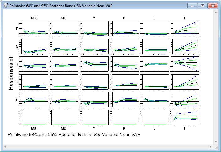
footer="Pointwise 68% and 95% Posterior Bands, Six Variable Near-VAR")

Output

The model is estimated using SUR since it doesn't have the same right-side variables in each equation.

Linear Systems - Estimation by Seemingly Unrelated Regressions

Iterations Taken 2

Quarterly Data From 1949:01 To 1989:03

Usable Observations 163

Log Likelihood 3590.3120

Dependent Variable FYGN3

Mean of Dependent Variable 0.0518561349

Std Error of Dependent Variable 0.0318224250

Standard Error of Estimate 0.0065462105

Sum of Squared Residuals 0.0069850182

Durbin-Watson Statistic 1.8425

Variable Coeff Std Error T-Stat Signif

*************************************************************************************

1. FYGN3{1} 1.134361652 0.080556800 14.08151 0.00000000

2. FYGN3{2} -0.639144328 0.129485544 -4.93603 0.00000080

3. FYGN3{3} 0.500220965 0.136348270 3.66870 0.00024379

4. FYGN3{4} -0.182773779 0.093808338 -1.94837 0.05137016

5. M1{1} 0.081932377 0.098342664 0.83313 0.40477054

6. M1{2} -0.224255124 0.163141065 -1.37461 0.16925279

7. M1{3} 0.303288259 0.152113094 1.99383 0.04617020

8. M1{4} -0.191669806 0.086888757 -2.20592 0.02738947

9. GNP82{1} 0.023662085 0.077602714 0.30491 0.76043233

10. GNP82{2} 0.040156577 0.099383392 0.40406 0.68617064

11. GNP82{3} -0.183734704 0.097935197 -1.87608 0.06064368

12. GNP82{4} 0.107979036 0.077350032 1.39598 0.16272076

13. GD{1} 0.123835892 0.104802738 1.18161 0.23736075

14. GD{2} 0.056931753 0.167766163 0.33935 0.73434471

15. GD{3} -0.156507372 0.164375202 -0.95213 0.34102855

16. GD{4} 0.015261957 0.101092923 0.15097 0.87999971

17. LHUR{1} 0.057724419 0.241062103 0.23946 0.81074991

18. LHUR{2} -0.028431465 0.373737652 -0.07607 0.93936076

19. LHUR{3} -0.204753887 0.379045986 -0.54018 0.58907140

20. LHUR{4} 0.030882172 0.237153047 0.13022 0.89639203

21. Constant 0.053493140 0.042626133 1.25494 0.20950139

22. GIN82{1} 0.068472294 0.027544549 2.48587 0.01292335

23. GIN82{2} -0.073264286 0.038683002 -1.89397 0.05822954

24. GIN82{3} 0.028652248 0.039015212 0.73439 0.46271316

25. GIN82{4} -0.011680214 0.026643826 -0.43838 0.66110828

Dependent Variable M1

Mean of Dependent Variable 5.4526945737

Std Error of Dependent Variable 0.5977479064

Standard Error of Estimate 0.0050988212

Sum of Squared Residuals 0.0042376704

Durbin-Watson Statistic 1.9320

Variable Coeff Std Error T-Stat Signif

*************************************************************************************

26. FYGN3{1} -0.634848867 0.064704306 -9.81154 0.00000000

27. FYGN3{2} 0.607372809 0.104004533 5.83987 0.00000001

28. FYGN3{3} -0.131023923 0.109516766 -1.19638 0.23154740

29. FYGN3{4} 0.018886109 0.075348120 0.25065 0.80208367

30. M1{1} 1.348249628 0.078990152 17.06858 0.00000000

31. M1{2} -0.213875817 0.131037100 -1.63218 0.10264208

32. M1{3} -0.178977827 0.122179285 -1.46488 0.14295403

33. M1{4} -0.013982105 0.069790220 -0.20034 0.84121096

34. GNP82{1} 0.002621955 0.062331545 0.04206 0.96644715

35. GNP82{2} 0.110083346 0.079826078 1.37904 0.16788246

36. GNP82{3} -0.079472337 0.078662869 -1.01029 0.31235620

37. GNP82{4} -0.049142585 0.062128587 -0.79098 0.42895458

38. GD{1} 0.034778698 0.084178970 0.41315 0.67949535

39. GD{2} -0.027236218 0.134752041 -0.20212 0.83982213

40. GD{3} 0.000598166 0.132028375 0.00453 0.99638513

41. GD{4} 0.054232469 0.081199197 0.66789 0.50420116

42. LHUR{1} -0.460004666 0.193624327 -2.37576 0.01751291

43. LHUR{2} 0.901261554 0.300191114 3.00229 0.00267955

44. LHUR{3} -0.493515747 0.304454839 -1.62098 0.10502155

45. LHUR{4} -0.066167753 0.190484521 -0.34737 0.72831674

46. Constant 0.048801088 0.034221253 1.42605 0.15385500

47. GIN82{1} -0.024391212 0.021880830 -1.11473 0.26496625

48. GIN82{2} 0.078614881 0.030532523 2.57479 0.01003005

49. GIN82{3} -0.078226568 0.030805347 -2.53938 0.01110483

50. GIN82{4} 0.055347179 0.021148990 2.61701 0.00887030

Dependent Variable GNP82

Mean of Dependent Variable 7.7256988534

Std Error of Dependent Variable 0.3655129025

Standard Error of Estimate 0.0086145804

Sum of Squared Residuals 0.0120963923

Durbin-Watson Statistic 1.7967

Variable Coeff Std Error T-Stat Signif

*************************************************************************************

51. FYGN3{1} -0.057773769 0.100577176 -0.57442 0.56568209

52. FYGN3{2} -0.248221974 0.161665935 -1.53540 0.12468546

53. FYGN3{3} 0.287662410 0.170234220 1.68980 0.09106552

54. FYGN3{4} -0.134807758 0.117122053 -1.15100 0.24973127

55. M1{1} 0.030469394 0.122783271 0.24816 0.80401378

56. M1{2} 0.123757295 0.203685693 0.60759 0.54345974

57. M1{3} -0.205421374 0.189916996 -1.08164 0.27941357

58. M1{4} 0.061462216 0.108482783 0.56656 0.57101184

59. GNP82{1} 0.982067830 0.096888927 10.13602 0.00000000

60. GNP82{2} 0.160262467 0.124082646 1.29158 0.19650318

61. GNP82{3} -0.163789959 0.122274539 -1.33953 0.18039940

62. GNP82{4} -0.000339649 0.096573446 -0.00352 0.99719384

63. GD{1} 0.115104542 0.130848835 0.87968 0.37903501

64. GD{2} -0.040533410 0.209460244 -0.19351 0.84655674

65. GD{3} -0.256257580 0.205226544 -1.24866 0.21179052

66. GD{4} 0.164787529 0.126217038 1.30559 0.19169249

67. LHUR{1} -0.214124501 0.300972055 -0.71144 0.47680968

68. LHUR{2} 0.746530957 0.466620790 1.59987 0.10962821

69. LHUR{3} -0.202784257 0.473248378 -0.42849 0.66829124

70. LHUR{4} -0.047325036 0.296091501 -0.15983 0.87301305

71. Constant 0.042104854 0.053267854 0.79044 0.42927292

72. GIN82{1} 0.060396904 0.035082906 1.72155 0.08515145

73. GIN82{2} -0.042876627 0.049815780 -0.86070 0.38940124

74. GIN82{3} -0.020920922 0.050214348 -0.41663 0.67694735

75. GIN82{4} 0.027452270 0.033981395 0.80786 0.41917017

Dependent Variable GD

Mean of Dependent Variable 3.8601005333

Std Error of Dependent Variable 0.5480266865

Standard Error of Estimate 0.0047092303

Sum of Squared Residuals 0.0036148265

Durbin-Watson Statistic 2.0535

Variable Coeff Std Error T-Stat Signif

*************************************************************************************

76. FYGN3{1} 0.189489949 0.060050494 3.15551 0.00160218

77. FYGN3{2} -0.118281110 0.096524079 -1.22541 0.22042258

78. FYGN3{3} 0.075997918 0.101639850 0.74772 0.45463043

79. FYGN3{4} -0.091101140 0.069928760 -1.30277 0.19265305

80. M1{1} 0.160237248 0.073308840 2.18578 0.02883145

81. M1{2} -0.164956080 0.121612348 -1.35641 0.17496908

82. M1{3} 0.044424698 0.113391625 0.39178 0.69521994

83. M1{4} -0.019324861 0.064770607 -0.29836 0.76542957

84. GNP82{1} 0.007044415 0.057848392 0.12177 0.90307821

85. GNP82{2} -0.028231042 0.074084644 -0.38106 0.70315525

86. GNP82{3} -0.071986175 0.073005097 -0.98604 0.32411195

87. GNP82{4} 0.088495861 0.057660032 1.53479 0.12483619

88. GD{1} 1.295165907 0.078124457 16.57824 0.00000000

89. GD{2} -0.108044540 0.125060095 -0.86394 0.38762032

90. GD{3} -0.162590521 0.122532327 -1.32692 0.18453535

91. GD{4} -0.059048232 0.075359001 -0.78356 0.43329886

92. LHUR{1} 0.214171361 0.179698033 1.19184 0.23332386

93. LHUR{2} -0.097546946 0.278600078 -0.35013 0.72623925

94. LHUR{3} 0.033575863 0.282557138 0.11883 0.90541117

95. LHUR{4} 0.009823515 0.176784055 0.05557 0.95568605

96. Constant -0.022334201 0.031757567 -0.70327 0.48188638

97. GIN82{1} -0.004014643 0.020272521 -0.19803 0.84301869

98. GIN82{2} 0.052905855 0.028259797 1.87212 0.06118940

99. GIN82{3} -0.029620898 0.028513868 -1.03882 0.29888647

100. GIN82{4} -0.006272017 0.019592114 -0.32013 0.74887002

Dependent Variable LHUR

Mean of Dependent Variable 0.0570695297

Std Error of Dependent Variable 0.0167072122

Standard Error of Estimate 0.0027801361

Sum of Squared Residuals 0.0012598526

Durbin-Watson Statistic 1.8212

Variable Coeff Std Error T-Stat Signif

*************************************************************************************

101. FYGN3{1} -0.006146236 0.032825868 -0.18724 0.85147435

102. FYGN3{2} 0.045972472 0.052763707 0.87129 0.38359602

103. FYGN3{3} -0.093616737 0.055560180 -1.68496 0.09199609

104. FYGN3{4} 0.083200414 0.038225701 2.17656 0.02951364

105. M1{1} -0.036394556 0.040073380 -0.90820 0.36377373

106. M1{2} -0.010453758 0.066477902 -0.15725 0.87504654

107. M1{3} 0.024413706 0.061984144 0.39387 0.69367689

108. M1{4} 0.015103243 0.035406060 0.42657 0.66969091

109. GNP82{1} -0.106195423 0.031622116 -3.35826 0.00078434

110. GNP82{2} 0.017278016 0.040497464 0.42664 0.66963835

111. GNP82{3} 0.059906917 0.039907343 1.50115 0.13331671

112. GNP82{4} 0.027645563 0.031519151 0.87710 0.38043032

113. GD{1} 0.002080696 0.042705778 0.04872 0.96114113

114. GD{2} -0.017574881 0.068362570 -0.25708 0.79711440

115. GD{3} 0.073267302 0.066980797 1.09386 0.27401843

116. GD{4} -0.048423168 0.041194076 -1.17549 0.23979928

117. LHUR{1} 1.174134997 0.098229730 11.95295 0.00000000

118. LHUR{2} -0.400219023 0.152293323 -2.62795 0.00859015

119. LHUR{3} -0.041766146 0.154456401 -0.27041 0.78684689

120. LHUR{4} 0.172371521 0.096636840 1.78370 0.07447177

121. Constant 0.022203504 0.017381799 1.27740 0.20146119

122. GIN82{1} -0.001911290 0.011400202 -0.16765 0.86685548

123. GIN82{2} 0.003227095 0.016149507 0.19983 0.84161648

124. GIN82{3} -0.007717547 0.016280729 -0.47403 0.63547881

125. GIN82{4} 0.006209713 0.011039059 0.56252 0.57376047

Dependent Variable GIN82

Mean of Dependent Variable 5.4930861728

Std Error of Dependent Variable 0.4432821202

Standard Error of Estimate 0.0259108781

Sum of Squared Residuals 0.1094338972

Durbin-Watson Statistic 1.9376

Variable Coeff Std Error T-Stat Signif

*************************************************************************************

126. Constant 0.009838916 0.025471195 0.38628 0.69929213

127. GIN82{1} 1.446070599 0.078112684 18.51262 0.00000000

128. GIN82{2} -0.464795005 0.137450841 -3.38154 0.00072082

129. GIN82{3} -0.007309488 0.137281274 -0.05324 0.95753701

130. GIN82{4} 0.025152776 0.078119689 0.32198 0.74746979

Covariance\Correlation Matrix of Residuals

FYGN3 M1 GNP82 GD LHUR GIN82

FYGN3 4.2853e-005 0.06777237 0.21129919 0.10058751 -0.37757048 0.32853059

M1 2.2621e-006 2.5998e-005 0.22777114 0.17783435 -0.21474695 0.16136926

GNP82 1.1916e-005 1.0005e-005 7.4211e-005 0.01139069 -0.63047513 0.48672522

GD 3.1009e-006 4.2701e-006 4.6210e-007 2.2177e-005 -0.15290033 0.11257864

LHUR -6.8715e-006 -3.0441e-006 -1.5100e-005 -2.0018e-006 7.7292e-006 -0.45875454

GIN82 5.5725e-005 2.1319e-005 1.0864e-004 1.3737e-005 -3.3047e-005 6.7137e-004

## NL6. NONLIN Parameter A12 Has Not Been Initialized. Trying 0

## NL6. NONLIN Parameter A21 Has Not Been Initialized. Trying 0

## NL6. NONLIN Parameter A23 Has Not Been Initialized. Trying 0

## NL6. NONLIN Parameter A24 Has Not Been Initialized. Trying 0

## NL6. NONLIN Parameter A31 Has Not Been Initialized. Trying 0

## NL6. NONLIN Parameter A36 Has Not Been Initialized. Trying 0

## NL6. NONLIN Parameter A41 Has Not Been Initialized. Trying 0

## NL6. NONLIN Parameter A43 Has Not Been Initialized. Trying 0

## NL6. NONLIN Parameter A46 Has Not Been Initialized. Trying 0

## NL6. NONLIN Parameter A51 Has Not Been Initialized. Trying 0

## NL6. NONLIN Parameter A53 Has Not Been Initialized. Trying 0

## NL6. NONLIN Parameter A54 Has Not Been Initialized. Trying 0

## NL6. NONLIN Parameter A56 Has Not Been Initialized. Trying 0

Covariance Model-Marginal Posterior - Estimation by BFGS

Convergence in 29 Iterations. Final criterion was 0.0000069 <= 0.0000100

Observations 163

Function Value 3856.6130

Prior DF 3.5000

Variable Coeff Std Error T-Stat Signif

************************************************************************************

1. A12 -0.631672606 0.368867847 -1.71246 0.08681134

2. A21 0.348463823 0.214584410 1.62390 0.10439695

3. A23 -0.201732085 0.080765034 -2.49777 0.01249790

4. A24 -0.245472883 0.118384690 -2.07352 0.03812402

5. A31 0.066098765 0.145360003 0.45472 0.64930740

6. A36 -0.167307846 0.026854301 -6.23021 0.00000000

7. A41 0.015087985 0.079542147 0.18969 0.84955565

8. A43 0.027267747 0.051141542 0.53318 0.59390763

9. A46 -0.026125504 0.016792250 -1.55581 0.11975394

10. A51 0.091762255 0.024822056 3.69680 0.00021833

11. A53 0.169559780 0.020426281 8.30106 0.00000000

12. A54 0.065962313 0.032983812 1.99984 0.04551765

13. A56 0.012818208 0.007155073 1.79149 0.07321544

Graph

The graph is probably too "busy" to be displayed in a 6 x 6 matrix (certainly at this size). Two things to note: the zero response of investment to the first five shocks is by construction. This is due to a combination of the other variables being excluded from the lags in the investment equation and the other shocks being excluded from the definition of the investment shock in the structural model. The other is that the misspecification of the dynamics of investment (which is treated as exogenous for illustration) causes it to be borderline unstable, and thus its shocks dominate all the responses.