SHORTANDLONGVECM.RPF

SHORTANDLONGVECM.RPF is an example of a VECM with short-and-long run restrictions for structural model. Adapted from Lütkepohl(2006), Example 9.4 from pp 377-383. It uses the @JOHMLE procedure for estimating the cointegrating vectors, the ECT instruction for setting up a VECM, @ShortAndLong procedure for doing the structural model for the covariance matrix and @VARIRF procedure for graphing impulse responses.

It's important to note that, because of the cointegration, the long-run response matrix is reduced rank. In this case, this is a three variable system with rank 2 cointegration (thus just one common trend). As a result, restricting the (1,2) and (1,3) long-run responses to zero (response of variable 1 (Y) to the final two shocks) also forces the other two variables to have zero long-run responses to shocks 2 and 3 as well. So three restrictions (in the pattern shown below) will just identify the model:

input lr

. 0 0

. . .

input sr

. . .

. . 0

. . .

As with all models of this type, the "shape" of the shocks is determined by the restrictions, but not the signs. And or all of the shocks can be sign-flipped and still achieve the same restrictions. To fully identify the shocks, you generally need some type of sign convention, such as positive or negative impact on one of the variables.

Full Program

open data kpswdata.rat
calendar(q) 1947
data(format=rats) 1947:1 1988:4 c in y mp dp r
*
* Data are already in logs. We need to scale by 100.
*
set c = c*100.0
set y = y*100.0
set in = in*100.0
*
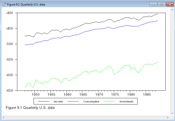
graph(footer="Figure 9.1 Quarterly U.S. data",$
key=below,klabels=||"Income","Consumption","Investment"||) 3
# y
# c
# in
*
* With two cointegrating vectors, this would be easier to analyze using
* CATS.
*
* This does the testing
*
@johmle(lags=2,det=constant)
# y c in
*
* This estimates given a chosen rank of 2 and defines two error
* correction equations and the beta matrix of cointegration vectors.
*
@johmle(lags=2,det=constant,rank=2,ect=ecteqns,vectors=beta)
# y c in
*
* Define and estimate the VECM
*
system(model=vecm)
variables y c in
det constant
lags 1 2
ect ecteqns
end(system)
*
estimate(resids=resids)
*
* Get the matrix of coefficients
*
compute vecmbeta=%modelgetcoeffs(vecm)
*
* Number of lags in the VECM (one more than the number of lags on the
* differences).
*
compute p=2
*
* Compute the sum of the coefficients on the short-run polynomial and
* the derivative of its z-transform evaluated at z=1.
*
compute lagsums=%identity(%nvar)
compute lagsumprime=%zeros(%nvar,%nvar)
do k=1,p-1
   ewise lagsums(i,j)=lagsums(i,j)-vecmbeta((j-1)*(p-1)+k,i)
   ewise lagsumprime(i,j)=lagsumprime(i,j)-k*vecmbeta((j-1)*(p-1)+k,i)
end do k
*
* Compute the long-run response matrix for the VECM.
*
compute masums=%perp(beta)*$
inv(tr(%perp(%vecmalpha))*lagsums*%perp(beta))*$
             tr(%perp(%vecmalpha))
*
dec rect lr(3,3) sr(3,3)
*
* Because of rank 2 cointegration, the masums matrix is rank one. As a
* result, restricting the (1,2) and (1,3) long-run responses to zero
* also forces the responses of the other two variables to zero as well.
* So three restrictions (in this pattern) will just identify the model.
*
input lr
. 0 0
. . .
. . .
input sr
. . .
. . 0
. . .
@ShortAndLong(lr=lr,sr=sr,masum=masums) %sigma f
disp ###.### "Impact Responses" f
disp ###.### "Long run Responses" masums*f
*
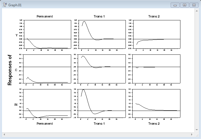
@varirf(factor=f,steps=30,model=vecm,shocklabels=||"Permanent","Trans 1","Trans 2"||)

Output

Likelihood Based Analysis of Cointegration

Variables: Y C IN

Estimated from 1948:01 to 1988:04

Data Points 164 Lags 4 with Constant

Unrestricted eigenvalues, -T log(1-lambda) and Trace Test

Roots Rank EigVal Lambda-max Trace Trace-95%

3 0 0.1597 28.5379 46.2592 29.3800

2 1 0.0870 14.9200 17.7213 15.3400

1 2 0.0169 2.8013 2.8013 3.8400

Cointegrating Vector for Largest Eigenvalue

Y C IN

0.261561 -0.380827 0.145438

Likelihood Based Analysis of Cointegration

Variables: Y C IN

Estimated from 1948:01 to 1988:04

Data Points 164 Lags 4 with Constant

Unrestricted eigenvalues, -T log(1-lambda) and Trace Test

Roots Rank EigVal Lambda-max Trace Trace-95%

3 0 0.1597 28.5379 46.2592 29.3800

2 1 0.0870 14.9200 17.7213 15.3400

1 2 0.0169 2.8013 2.8013 3.8400

Cointegrating Vector for Largest Eigenvalue

Y C IN

0.261561 -0.380827 0.145438

VAR/System - Estimation by Cointegrated Least Squares

Quarterly Data From 1948:01 To 1988:04

Usable Observations 164

Dependent Variable Y

Mean of Dependent Variable 0.4182890244

Std Error of Dependent Variable 1.3707599780

Standard Error of Estimate 1.1590151009

Sum of Squared Residuals 204.18403262

Durbin-Watson Statistic 1.9756

Variable Coeff Std Error T-Stat Signif

************************************************************************************

1. D_Y{1} 0.141023460 0.113718190 1.24011 0.21684440

2. D_Y{2} 0.099838231 0.116756200 0.85510 0.39384159

3. D_Y{3} 0.073693248 0.109225396 0.67469 0.50089786

4. D_C{1} 0.111093267 0.152540031 0.72829 0.46755703

5. D_C{2} 0.017209588 0.153212347 0.11233 0.91071386

6. D_C{3} -0.138757567 0.144123302 -0.96277 0.33719219

7. D_IN{1} 0.126982268 0.053607388 2.36875 0.01910549

8. D_IN{2} 0.006400891 0.053306090 0.12008 0.90457990

9. D_IN{3} -0.028470876 0.050436852 -0.56449 0.57325576

10. Constant 0.465282470 4.428459154 0.10507 0.91646160

11. EC1{1} -0.349832174 0.090503874 -3.86538 0.00016391

12. EC2{1} -0.218503306 0.090503874 -2.41430 0.01695404

Dependent Variable C

Mean of Dependent Variable 0.4714621951

Std Error of Dependent Variable 0.8013465549

Standard Error of Estimate 0.7425875804

Sum of Squared Residuals 83.818319813

Durbin-Watson Statistic 2.0249

Variable Coeff Std Error T-Stat Signif

************************************************************************************

1. D_Y{1} 0.143581803 0.072859892 1.97066 0.05057965

2. D_Y{2} 0.008807177 0.074806363 0.11773 0.90643466

3. D_Y{3} -0.150455995 0.069981334 -2.14994 0.03314143

4. D_C{1} -0.171789663 0.097733267 -1.75774 0.08080480

5. D_C{2} 0.165945845 0.098164024 1.69050 0.09298285

6. D_C{3} 0.077392687 0.092340621 0.83812 0.40327831

7. D_IN{1} 0.025870481 0.034346559 0.75322 0.45248339

8. D_IN{2} 0.011210152 0.034153516 0.32823 0.74319073

9. D_IN{3} 0.061106397 0.032315178 1.89095 0.06053379

10. Constant -5.305298797 2.837339018 -1.86981 0.06343286

11. EC1{1} -0.165121019 0.057986348 -2.84758 0.00501502

12. EC2{1} 0.036035252 0.057986348 0.62144 0.53523861

Dependent Variable IN

Mean of Dependent Variable 0.4194365854

Std Error of Dependent Variable 2.8403281403

Standard Error of Estimate 2.2323442565

Sum of Squared Residuals 757.47085370

Durbin-Watson Statistic 2.0136

Variable Coeff Std Error T-Stat Signif

************************************************************************************

1. D_Y{1} 0.79907476 0.21902920 3.64826 0.00036228

2. D_Y{2} 0.19869699 0.22488062 0.88357 0.37832560

3. D_Y{3} 0.00989003 0.21037576 0.04701 0.96256597

4. D_C{1} -0.25168997 0.29380278 -0.85666 0.39297972

5. D_C{2} -0.04078897 0.29509771 -0.13822 0.89024799

6. D_C{3} 0.02941480 0.27759157 0.10596 0.91575039

7. D_IN{1} 0.27748084 0.10325158 2.68742 0.00800286

8. D_IN{2} -0.04582821 0.10267126 -0.44636 0.65597340

9. D_IN{3} 0.02436742 0.09714491 0.25084 0.80227985

10. Constant -25.77546676 8.52952248 -3.02191 0.00294834

11. EC1{1} -0.93123390 0.17431680 -5.34219 0.00000033

12. EC2{1} 0.05058377 0.17431680 0.29018 0.77207177

Impact Responses

0.316 0.558 0.913

0.595 0.396 -0.000

-0.171 2.089 0.473

Long run Responses

0.700 0.000 -0.000

0.745 0.000 -0.000

0.691 0.000 -0.000

Graphs