SPECTRUM.RPF

SPECTRUM.RPF is an example of calculation of a spectral density. It is adapted from Brockwell & Davis(1991) (their) Example 10.4.3. It uses the @SPECTRUM procedure to do the calculations.

Full Program

open data sunspots.dat
calendar 1770
data(format=free,org=columns) 1770:1 1869:1 sunspots
*
diff(center) sunspots / cspots
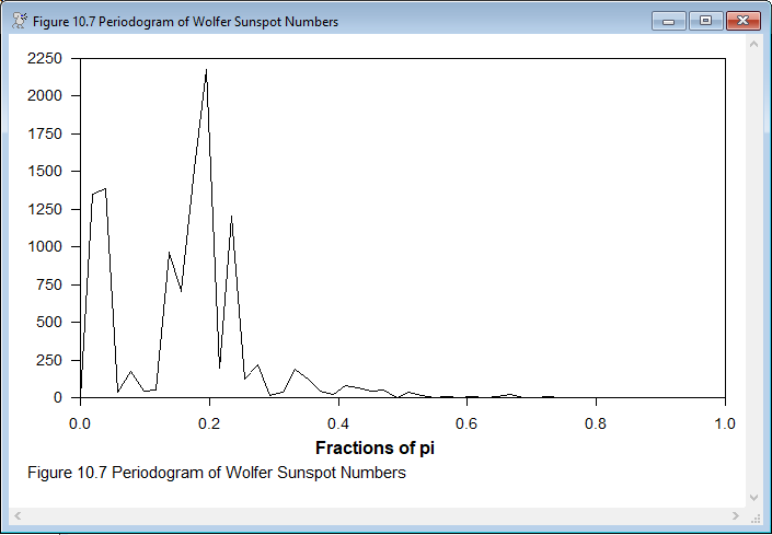
@spectrum(footer="Figure 10.7 Periodogram of Wolfer Sunspot Numbers",$
periodogram,nologscale) cspots
@spectrum(footer="Figure 10.8 Spectral Estimate of Wolfer Sunspot Numbers",$
weights=||3.0,3.0,2.0,1.0||,nologscale,spectrum=smoothed,ordinates=128) cspots
*
* Confidence bands (text only does these for the artificial data). %EDF
* is the Equivalent Degrees of Freedom of the window used by @spectrum.
*
set lower = smoothed*%edf/%invchisqr(.025,%edf)
set upper = smoothed*%edf/%invchisqr(.975,%edf)
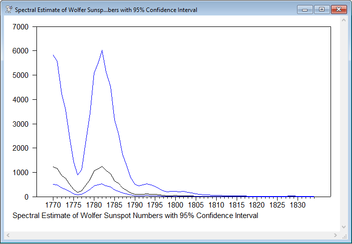
graph(footer="Spectral Estimate of Wolfer Sunspot Numbers with 95% Confidence Interval") 3
# smoothed
# lower / 2
# upper / 2
*
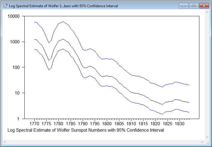
* Same thing done on log scale - the confidence bands are equal width
*
graph(footer="Log Spectral Estimate of Wolfer Sunspot Numbers with 95% Confidence Interval",log=10) 3
# smoothed
# lower / 2
# upper / 2

Graphs

This shows the periodogram (an unsmoothed estimate of the spectrum with a high variance), a smoothed estimate (trades some bias for a large reduction in variance), plus graphs of the smoothed spectrum with confidence bands, one in regular scale, one in log scale. Note that the confidence bands are fixed width in the log scale.