SPECFORE.RPF

SPECFORE.RPF is an example of the use of the @SPECFORE procedure for forecasting univariate time series using spectral methods.

This uses the same series (U.S. interest rate spread) as in the ARIMA.RPF example. That identified a fairly complicated ARMA(2,(1,7)) model—this estimates that model and does 24 forecast periods doing a holdback of the last 24 periods of data:

boxjenk(constant,ar=2,ma=||1,7||,define=armaeq) $

spread 1961:4 2006:1

uforecast(equation=armaeq,from=2006:2,to=2008:1) armafore

This does the same thing using @SPECFORE. This is fit using all data prior to the forecast period (2006:2 to 2008:1).

@specfore spread 2006:2 2008:1 spfore

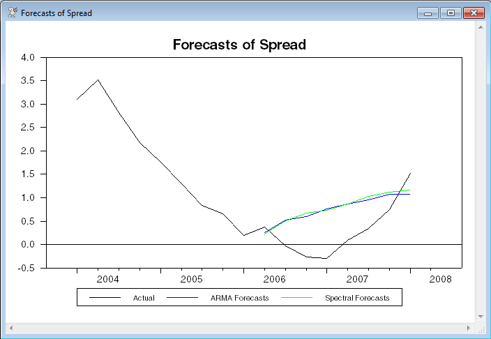
This does a graph of the two forecasts with the actual data for both the forecast period and the two years before that:

graph(header="Forecasts of Spread",key=below,klabels=||"Actual","ARMA Forecasts","Spectral Forecasts"||) 3

# spread 2004:1 2008:2

# armafore

# spfore

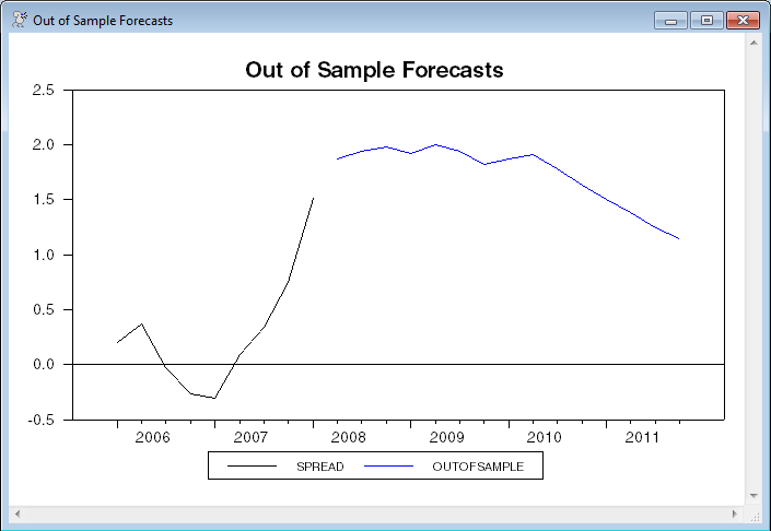
This computes and graphs out-of-sample forecasts. (This will re-do estimates using data through 2008:1, which is the end of data).

@specfore spread 2008:2 2009:12 outofsample

graph(key=below,header="Out of Sample Forecasts") 2

# spread 2006:1 2008:1

# outofsample

Full Program

open data quarterly.xls
calendar(q) 1960:1
data(format=xls,org=columns) * 2008:1 tbill r10
*
* Compute spread
*
set spread = r10 - tbill
*
* Forecasts with ARMA(2,(1,7)) model, holding back the last
* two years of data.
*
boxjenk(constant,ar=2,ma=||1,7||,define=armaeq) $
spread 1961:4 2006:1
uforecast(equation=armaeq,from=2006:2,to=2008:1) armafore
*
* Forecasts with @SPECFORE procedure
*
@specfore spread 2006:2 2008:1 spfore
*
graph(header="Forecasts of Spread",key=below,klabels=$
||"Actual","ARMA Forecasts","Spectral Forecasts"||) 3
# spread 2004:1 2008:2
# armafore
# spfore
*
* Compute and graph out-of-sample forecasts
*
@specfore spread 2008:2 2009:12 outofsample
graph(key=below,header="Out of Sample Forecasts") 2
# spread 2006:1 2008:1
# outofsample

Output

Box-Jenkins - Estimation by LS Gauss-Newton

Convergence in 15 Iterations. Final criterion was 0.0000092 <= 0.0000100

Dependent Variable SPREAD

Quarterly Data From 1961:04 To 2006:01

Usable Observations 178

Degrees of Freedom 173

Centered R^2 0.8198522

R-Bar^2 0.8156869

Uncentered R^2 0.9234253

Mean of Dependent Variable 1.4226226011

Std Error of Dependent Variable 1.2266825607

Standard Error of Estimate 0.5266357095

Sum of Squared Residuals 47.980714503

Log Likelihood -135.8934

Durbin-Watson Statistic 1.9459

Q(36-4) 30.1181

Significance Level of Q 0.5620416

Variable Coeff Std Error T-Stat Signif

************************************************************************************

1. CONSTANT 1.401401285 0.334894151 4.18461 0.00004536

2. AR{1} 0.316457693 0.103639768 3.05344 0.00262001

3. AR{2} 0.482419889 0.101684794 4.74427 0.00000436

4. MA{1} 0.863154737 0.061556875 14.02207 0.00000000

5. MA{7} -0.146596834 0.037887076 -3.86931 0.00015441

Graphs