While COMPUTE and DISPLAY are important, if you’re getting started with RATS, you probably have some time series data that you want to use. There are three main types of data collection: time series, cross section/survey, and panel/longitudinal. While RATS can handle all three, its specialty is time series data, and the specialized techniques used in working with it. In this example, we introduce some basic tools for working with time series data. The CALENDAR instruction discussed here is provided on the file ExampleTwo.rpf (everything else in this section is done using menu operations).

 

In time series data, the basic unit of data is a time series, which is a time sequence of data that (usually) has a specific starting place in time and a specific reporting frequency. What makes time series data very different from other forms is that the data you use may come from many sources—in the U.S., the Census Bureau, the Federal Reserve and the Bureau of Labor Statistics (among many others) are each the original sources of key data series. Time series can start at different times; in some cases, they can end rather abruptly (such as exchange rates involving Euro zone countries).

 

The Calendar Wizard

To work with time series data, we first want to tell RATS the frequency and starting date for our data set. One way to do that is to use the Calendar Wizard. Select the the Data/Graphics—Calendar operation. RATS will display the Calendar Wizard dialog box shown below, which allows you to set frequency and date information. The most common frequencies are in the “Standard Frequencies” group.

 

 

 

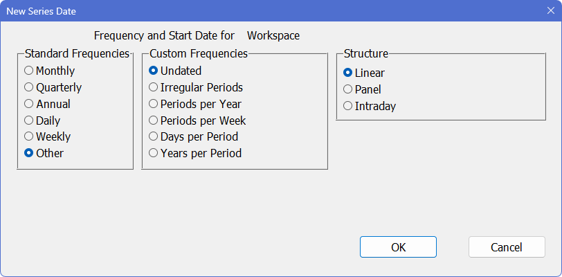
In this case, we want quarterly data, beginning in the first quarter of 1998, so click on the “Quarterly” button and change the “Year” field to read 1998, like this:

 

 

Now click on “OK”. RATS will generate the corresponding CALENDAR instruction:

 

CALENDAR(Q) 1998:1

 

in the input window and execute it automatically. The Q in parentheses stands for “quarterly”. This is called an option, and this option tells RATS that we will be working with quarterly data. When you use options for an instruction, the left parentheses must appear immediately after the instruction name, with no spaces in between.

 

The date 1998:1 tells RATS that our data begin in the first quarter of 1998. This value is called a parameter. The parameters generally are information that is either necessary or very commonly used, while the options are just that—something that you might or might not use.

 

Note that you generally do not need to use the Calendar Wizard if you intend to use one of the Data Wizards (in Example Three) to read data in from a file, since they will set the date scheme themselves.

Creating a Data Series

If at all possible, you do not want to type in data. Most of your work will be done using data read in from files or database connections, but for now, we’ll have you type in some numbers to introduce you to tools for creating, viewing, and editing data.

 

First, open the Data/Graphics—Create Series (Data Editor) menu operation. RATS will display an empty Series Edit Window. As this is a new series, the first cell shows “NA”, for “Not Available”. We use the NA abbreviation both in RATS output and in the manuals to signify a missing value.

 

Here are the numbers to enter (data for 1998 in row one, for 1999 in row two, etc.):

 

98.2 100.8 102.2 100.8

99.0 101.6 102.7 101.5

100.5 103.0 103.5 101.5

 

Start by typing the first number (98.2) into the cell at the top. Then, hit the right arrow key. This saves the value you typed in and moves to the next cell. Type in the second number (100.8), hit the right arrow key again, and so on. Note that the right arrow still works when you get to the end of a “line”. Because this is a time series, the lines are just to help organize your view of the data—what we really have is a continuous sequence of values. When you get to the final value, just hit <Enter> (rather than the right arrow) to save the value.

 

If you only want to type in a few of the values, that’s fine—everything we discuss below will still work, although the results will look different. You can also copy and paste the data lines above into the editor.

 

If you need to edit a value, click on (or navigate to) the cell you want to change, edit the value, and hit <Enter>.

 

Once you are done, the window should look like this:

 

The View Menu

The operations on the View menu provide ways to quickly examine data series and other variables. These operations do not generate RATS instructions the way the wizards do. However, they are very handy for verifying your data and doing some “quick glance” analysis before beginning work in earnest.

 

The second most common error that we’ve found in replicating examples (and the one that is probably most significant in practice) is where a data set is simply wrong—for instance, the data are for a different set of years than the author thought. And these are for papers which have been circulated, presented in seminars, peer-reviewed and published. Do yourself a favor: make sure your data are what you think they are before doing any major work with them. The View menu can help with this.

 

Try the View—Time Series Graph operation (or click on the  toolbar item). You’ll see a simple graph of the data. This is not intended to be a “production” graph; instead, it’s a quick line graph of the data that can help you spot any obvious errors like missing a decimal point. If you see that you have a value that’s clearly wrong, you should be able to go back to the series editor window and use the  or  toolbar icons, which move to the maximum and minimum values in the series, respectively, to correct the problem.

 

While there are several other “quick-view” operations (the ones at the bottom of the View menu), the other one that is very handy is View—Statistics. If you choose this (or the  icon), you will see a new type of window called a report that looks like this:

 

Report Windows

A Report Window is like a read-only spreadsheet. The descriptive text and values are arranged in columns, with longer strings covering (“spanning”) several columns. Output from RATS will either be in the form of Report Windows or text in the Output Window, and sometimes both. You can copy information out of a Report Window and paste it into a spreadsheet or word processing program.

 

Test Results

The report for Statistics includes four different “tests”: the t-statistic, skewness, kurtosis, and Jarque-Bera. For each of these, the left column gives the test statistic and the right gives the marginal significance level (also known as the p-value). This is the probability that a random variable with the appropriate distribution will exceed the computed value (in absolute value for Normal and t). Wherever possible, RATS will compute the significance level for tests, which allows you to avoid using “lookup tables” for critical values. You reject the null if the marginal significance level is smaller than the significance level you want. For instance, a marginal significance level of .03 would lead you to reject the null hypothesis if you are testing at the .05 level (.03<.05), but not if you are testing at the .01 level. Here, the only of the four that we would “reject” under standard procedures is Mean=0, which has a test statistic so far out in the tails that the p-value shows as just being 0. (If you paste it into a spreadsheet, you’ll find that it’s actually roughly \(10^{-21}\).)

 

This would be a good time to warn you about over-interpreting test results. RATS will often compute tests and summary statistics which might be useful. It’s up to you to decide whether they actually make any sense in particular situation. The three test statistics here that “pass” are all tests for the Normal distribution (the “excess” in excess kurtosis is the difference between the sample value and what would be expected if the data were from a Normal population). Should we therefore conclude that the data are from a Normal population? Absolutely not. Those are all test statistics computed under the assumption that the observations are independent. This is our raw time series data—we certainly don’t expect it to be independent, and from the graph it’s clear that it has a bit of a trend and a rather pronounced seasonal. If we were looking at the statistics on the residuals from an estimated model, then those last three tests might be interesting; here, they aren’t. Some other software packages actually do many more of these “automatic” tests than RATS, which has led people misusing them to conclude that a model that made no sense at all was fine because it “passed” all the “tests”.

 

Saving the Data

You may have noticed that we haven’t yet talked about saving the data. If you do File—Save, you will be prompted for a series name (and comments), or if you do File—Close or click the "close" button on the window, you will first be asked if you want to save the changes; if you answer “yes”, you will be asked the same question about the name and comments:

 

 

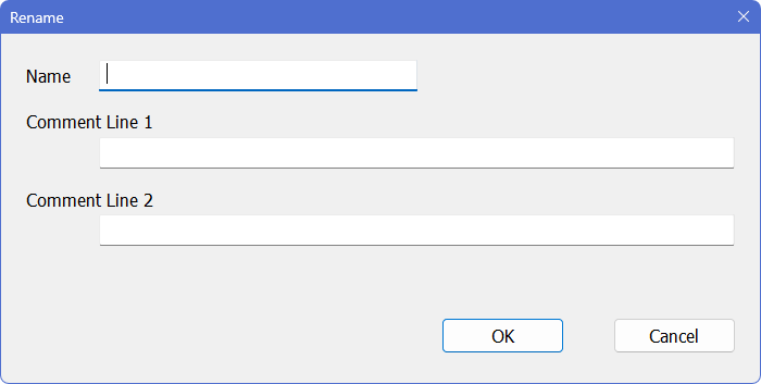
For our purposes, enter QUARTER as the name as shown above. Leave the comments blank.

 

If you do the menu operation View—Series Window, you will now see a Series Window listing all the series in memory. We’ll talk more about this when we have more data. For now, this should just have one line for the series QUARTER. At this point, we have saved the data out of the Series Edit Window into a RATS series. If you need a permanent copy, you need to take one more step: exporting the data to a file, which can be done with File—Export or File—Save As.

Series Names

Series (and other variable) names in RATS can be from one to sixteen characters long. They must begin with a letter (or %, though you should generally avoid those, as they’re used for names reserved by RATS), and can consist of letters, numbers, and the _ , $ and % symbols. Variable names aren’t case-sensitive.

 

Generally, you’ll want to choose names which are just long enough so you will know what each represents. In most cases, your data files will include names for the series stored on the file, and RATS will use those names when it reads in the data. Thus, the series names on the file should conform to the restrictions described above.

 

Learn More: Series Edit Windows

Learn More: Report Windows

 

Copyright © 2025 Thomas A. Doan