In this section, we will work with a sample data set from Pindyck and Rubinfeld(1998) to demonstrate a variety of tasks, including data transformations and multiple regression models.

  

All of the commands that we will describe here are also provided for you in a RATS program file called ExampleThree.rpf.

 

We recommend that you begin by entering the commands yourself as we discuss them. However, if you encounter difficulties, you can refer to (or execute the instructions on) ExampleThree.rpf to see exactly how things should look.

 

The sample data set is provided on an XLS (Excel) spreadsheet called ExampleThree.xls. The following data series are provided on the file:

 

 

Our primary goal will be to fit the following regression models to these data:

\begin{equation} Rate_t = \alpha + \beta _1 IP_t + \beta _2 \left( {M1_t - M1_{t - 3} } \right) + \beta _3 PSUM_t + u_t \end{equation}

where

\begin{equation} PSUM_t = \frac{{\Delta PPI_t }}{{PPI_t }} + \frac{{\Delta PPI_{t - 1} }}{{PPI_{t - 1} }} + \frac{{\Delta PPI_{t - 2} }}{{PPI_{t - 2} }} \end{equation}

and

\begin{equation} Rate_t = \alpha + \beta _1 IP_t + \beta _2 GRM2_t + \beta _3 GRPPI_{t - 1} + u_t \end{equation}

where

\begin{equation} GRM2_t = \frac{{\left( {M2_t - M2_{t - 1} } \right)}}{{M2_{t - 1} }} \text{ and } GRPPI_t = 100\frac{{\left( {PPI_t - PPI_{t - 1} } \right)}}{{PPI_{t - 1} }} \end{equation}

 

Our data were taken from Haver Analytics’ USECON database. The Haver series names for these are FTB3, IP, FM1, FM2, and PA, respectively. We’ve converted them to the names shown above for our example. The series begin in January, 1959, and run through September, 1999. Some of the values are slightly different than the older data used in Pindyck and Rubinfeld.

 

Here’s a portion of the data on the file:

 

Date        IP       M1        M2         PPI        RATE

1959:01     36.000   138.900   286.700    31.700     2.84

1959:02     36.700   139.400   287.700    31.700     2.71

1959:03     37.200   139.700   289.200    31.700     2.85

1959:04     38.000   139.700   290.100    31.800     2.96

1959:05     38.600   140.700   292.200    31.800     2.85

1959:06     38.600   141.200   294.100    31.700     3.25

1959:07     37.700   141.700   295.200    31.700     3.24

1959:08     36.400   141.900   296.400    31.600     3.36

1959:09     36.400   141.000   296.700    31.700     4.00

1959:10     36.100   140.500   296.500    31.600     4.12

1959:11     36.300   140.400   297.100    31.500     4.21

1959:12     38.600   140.000   297.800    31.500     4.57

 

Getting the Data In

As in our previous example, we want to start by defining a date scheme and then reading data into memory. In this case, though, we’ll be reading the data from a file, which is much more common. We could just type in the necessary instructions, but another option is to use the Data Wizard to do this.

 

The Data Wizard approach is usually preferable for most file formats. However, for certain file formats, or in cases where you need to pull in data from multiple sources, you may need to type the instructions directly.

 

A Clean Slate—The Clear Memory Operation

If you still have RATS running after completing the previous example, you will probably want to clear the memory of the settings and data entered earlier. You can do that by using the File—Clear Memory operation, or clicking on the “Clear Memory” toolbar icon: . You can also close the Input Window, then open a new one using the menu operation File–New-Editor/Text Window.

 

Any of these will clear any data series and other variables, as well as any settings defined by instructions like CALENDAR, from memory. This allows you to start fresh, as if you had never executed any instructions. Note that Clear Memory does not delete any text or close any windows.

 

The Data Wizard

RATS actually offers two Data Wizards—one for use with RATS format data files, and one for all other file types. We’ll discuss the wizard for RATS format data files in Example Six. For now, select the Data (Other Formats) from the Data/Graphics menu.

 

We will be working with an Excel “XLS” format file called ExampleThree.xls, so select “Excel 3.0-2003 Files (*.XLS)” from the drop-down list of file types. The dialog box should now show files with that extension in the current directory.

 

The default start-up directory for RATS should be the directory containing the main example programs, data files, and procedures that ship with RATS, including ExampleThree.xls. So, you should see as one of the files listed in the dialog box. If not, you can use the dialog box to navigate to the appropriate directory for Windows or Macintosh.

 

Select ExampleThree.xls and click the “Open” button. RATS will display the Data Wizard dialog box. Click on the “Scan” button, which scans the date information on the file to determine the appropriate CALENDAR setting.

 

You should see something like this:

 

Data Organization

The “Data Organization” section tells RATS how the data are arranged on the file. Here, the data series run down the page in columns, so we want to use the “Down Page” setting (which is, by far, the most common and should be selected by default).

 

You only need to use the “Header Rows” field if you need to skip lines (other than a row of series names) at the top of file, such as lines of text describing the contents of the file. Our data file begins with the series labels (which we need) on row 1, so we leave “Header Rows” set to zero.

 

Similarly, you can use “Columns to Skip” if you want RATS to ignore columns at the left of the file. The “Bottom Row” and “Right Column” fields default to the last row and column numbers found in the file. You can reduce these values to skip rows at the bottom or columns at the right. For this example, leave these set to the default values.

 

If you are reading a spreadsheet file containing data on multiple sheets, the “Sheet” field will let you pick which sheet you want to read. If you change sheets, the preview table will reload and the “Bottom Row” and “Right Column” fields will reset.

Date/Calendar Handling

The “Format of Date Strings” field shows what RATS thinks is the format of the date information on the file (if any). If it thinks there is more than one possible interpretation, you can use this field to select from the choices it offers. Here, RATS has correctly guessed that the dates are in the “year:month” form (abbreviated “y:m”).

 

The “File Dates” field describes the frequency and starting date of the data as it appears on the file. When you click on “Scan”, RATS examines the file to determine the frequency and starting date of the data set. In this case, it should report that the data is monthly, starting in January of 1959.

 

The “Target Dates” field shows the starting date and frequency that will be used in your RATS session. By default, this will match the “File Dates” setting. You can set or change it by clicking on the “Set” button. This is useful if you only want to read in a subset of the data, or if you want to work with the data at a different frequency.

 

If you set a different target frequency, RATS will automatically compact or expand the data to that frequency. The “Compact by” box allows you to select the compaction method that will be used when going to a lower frequency. That will only be active if the “File Dates” and “Target Dates” have a different frequency.

 

Read the Data

For now, accept the default settings and click on “OK”. This will put up the following dialog, which is designed to allow you to provide or change the working names for the series on the data file. If, as in this case, the series names on the file are what you want, you can click on "OK for All". A more detailed description of the name dialog is provided in the description of the wizard.

 

 

 

RATS will generate and execute the appropriate CALENDAR, OPEN DATA, and DATA commands. They should look something like this:

 

OPEN DATA "C:\Users\Public\Documents\WinRATS\ExampleThree.xls"

CALENDAR(M) 1959:1

DATA(FORMAT=XLS,ORG=COLUMNS) 1959:01 1999:09 RATE IP M2 M1 PPI

 

Let’s take a closer look at each of these.

 

The OPEN Instruction

OPEN DATA "C:\Users\Public\Documents\WinRATS\ExampleThree.xls"

 

The OPEN DATA instruction tells RATS the name and location of the data file you want to read. This instruction includes the full path to the file (which may be slightly different on your system). If you are typing in the instruction directly, you can leave out the path if the file is located in the default directory. 

 

The CALENDAR Instruction

CALENDAR(M) 1959:1

 

The CALENDAR instruction is similar to the one in our previous example, but here we have the option M for monthly data, rather than Q for quarterly, and the data start in January of 1959.

 

Some of the Pindyck and Rubinfeld examples apply only to data from November, 1959. We will use “date parameters” to skip earlier observations when necessary in this example, but another alternative would be to set our CALENDAR to start in November. We could do that in the Data Wizard by clicking on the “Set” button under “Target Dates” and replacing the “1” in the “Month/Period” cell with “11” (for the 11th month), the resulting CALENDAR would be:

 

CALENDAR(M) 1959:11

 

With this setting, RATS would skip the data for January through October, and start reading in data beginning with the November 1959 observation.

 

If you have cross-sectional data, with no time series periodicity, omit the CALENDAR instruction.

 

Working with Dates

To refer to a date in RATS, use the following formats:

 

          

With annual data, period is always one, so any reference to a date in annual data must end with :1. The :1 after the year is very important, because without it, RATS will assume you are specifying an entry number, not a date.

 

 

The DATA Instruction

 

DATA(FORMAT=XLS,ORG=COLUMNS) 1959:01 1999:09 RATE IP M2 M1 PPI

 

This reads the data series RATE, M1, M2, IP, and PPI from the file.

 

Here, we have two options, separated by commas: FORMAT and ORGANIZATION. You can abbreviate option names to three or more characters, which is what we did with the ORG option. Recall that the list of options must appear immediately after the instruction name, with no space between the instruction and the left parenthesis.

 

For now, we’ll go over these two options quickly. Because the data step is so important, we included a full "Dealing with Data" section; if you need more detail, you can check that out.

The FORMAT Option

FORMAT gives the format of the file you are reading. As noted above, ExampleThree.xls is an Excel spreadsheet file, and the option for that is FORMAT=XLS. RATS supports about 20 formats.

 

Note: RATS does not try to determine the format of the file based on the file name or extension—the FORMAT option must be set to match the format of the file being read.

 

The ORGANIZATION Option

The ORG option describes how the data are arranged on the file. The “Down Page” setting on the wizard corresponds to the setting ORG=COLUMNS while the “Across Page” setting corresponds to ORG=ROWS. You can also abbreviate the choices for options like this to three or more characters. For example: ORG=COL.

 

The Entry Range

The first two parameters (1959:01 and 1999:09) specify the starting and ending dates to be read in. You will generally omit explicit date ranges and just let RATS figure out the appropriate range for a given operation. Here, though, the wizard includes the dates so that you know (and have a record of) the exact range being read.

 

The Series Names

For files that include series names (which RATS requires for most formats), listing the series names on the DATA instruction is optional—if you omit the list, RATS reads in all the series on the file. If you do provide a list, RATS reads only those series.

 

For text files without any series names (which can be handled with FORMAT=FREE), you must supply a list of series names if typing in the DATA instruction yourself (otherwise RATS would have no way to identify the data). If you use the Data Wizard, RATS will prompt you for names. The series list is also required when reading some database formats, to avoid accidentally reading a huge number of series.

 

Check the Data

First, we need to verify that the data have been read in properly. To begin, select the View—Series Window operation. You’ll see a window displaying a list of all the series:

 

 

This provides a quick check on the number of observations in each series, as well as the frequency and data range. Now, select (highlight) all of the series in the window ( toolbar or Edit—Select All) and then select View—Statistics or click on the “Basics Statistics” toolbar icon: . You should see the following table of summary statistics for each series. The most important items to check are the number of observations (Obs) and the minimum and maximum values. Be sure they are reasonable given what you know about the data. A particular “red flag” is a minimum of 0 for a series that shouldn’t have zero values (GDP for instance), which is a result of a data set using 0 to mean “missing”.

 

 

You can explore the other View menu (and toolbar button) operations introduced in Example Two with combinations of one or more series—just highlight the series you want to include before selecting an operation.

 

Another way to generate the table of statistics is to use the instruction TABLE. Type in the following and hit <Enter>:

 

table

 

The results should appear in the output window, and match those shown in the Statistics window above.

 

STATISTICS and the Univariate Statistics Wizard

For a more detailed set of sample statistics, you can use STATISTICS instruction with a single series:

 

statistics rate

 

Here’s resulting output:

 

Statistics on Series RATE

Monthly Data From 1959:01 To 1996:02

Observations                446

Sample Mean            6.058587      Variance            7.701206

Standard Error         2.775105      of Sample Mean      0.131405

t-Statistic (Mean=0)  46.106212      Signif Level        0.000000

Skewness               1.186328      Signif Level (Sk=0) 0.000000

Kurtosis (excess)      1.587381      Signif Level (Ku=0) 0.000000

Jarque-Bera          151.440700      Signif Level (JB=0) 0.000000

 

 

The corresponding wizard is the Statistics—Univariate Statistics operation. If you select that operation, RATS will display the following dialog box:

 

 

The first step is to select the series you want to use from the “Series” drop-down list—here, we’ve selected the series RATE.

 

Next, click on one or more of the “Basic Statistics”, “Extreme Values”, or “Autocorrelations” check boxes. Here, we’ve selected “Basic Statistics”, which generates a STATISTICS command as shown above.

 

“Extreme Values” generates an EXTREMUM instruction, which reports the maximum and minimum values of the series. “Autocorrelations” generates a CORRELATE instruction, which computes autocorrelations (and partial autocorrelations if you provide a series for the “Partial Corrs” field). You can check any combination of these three boxes. The other fields allow you to select the range used for the computations and to select various options for the autocorrelation computations.

 

Data Transformations and Creating New Series

The SET Instruction

In most of your work with RATS, you will need to do at least a few data transformations, and you will often need to create new series from scratch. You can do that using the SET instruction, or one of several wizards. For our example, we need to define quite a few new series. We’ll start by generating a couple of differenced series using SET. Execute the following instructions:

 

set ppidiff = ppi - ppi{1}

set m1diff = m1 - m1{3}

 

Be sure to put at least one blank space before the = sign.

 

Let’s examine the first transformation. The {1} notation (which we refer to as “lag notation”) tells RATS to use the first lag of PPI in the transformation. This creates a new series called PPIDIFF, and sets it equal to the first difference of PPI:

 

          \(\text{PPIDIFF}_t  =  (\text{PPI}_t – {PPI}_{t–1})\)  for each entry \(t\) in the default entry range.

 

Note that PPIDIFF cannot be defined for 1959:1, because we do not have data for 1958:12, which would be the one period lag from 1959:1. RATS recognizes this, and defines entry 1959:1 of PPIDIFF to be a missing value.

 

Similarly, M1DIFF is defined as the three-lag difference of the series M1, so that \(\text{M1DIFF}_t = \text{M1}_t – \text{M1}_{t–3}\). M1DIFF will be defined starting in 1959:4.

 

If you want to see the values of these series, click on or re-open the Series Window, highlight the series you want to view, and click on View—Data Table (or click on the  icon).

 

Next, we’ll create some quarter to quarter growth rates, again using the “{L}” lag notation, and the “/ ” division operator:

 

set grm2  = (m2 - m2{1})/m2{1}

set grppi = (ppi - ppi{1})/ppi{1}

 

We also need to create a three-period moving average term. First, we define PRATIO as the ratio of PPIDIFF (the first difference of PPI that we created above) to PPI. Then, we define PPISUM as the sum of the current and two lags of PRATIO. This could be done with a single SET, but is easier to read or modify this way:

 

set pratio = ppidiff/ppi

set ppisum = pratio + pratio{1} + pratio{2}

 

Note that there are specialized instructions that can be used for some of these operations, such as DIFFERENCE and FILTER, but SET is the most important because it is the most flexible.

 

Data Transformation and Related Wizards

RATS offers several wizards for doing transformations, creating dummy variables, and other data-related operations. The Data/Graphics—Transformations operation is probably the most versatile.

 

For example, another way to create PPIDIFF as the first difference of PPI is to select Data/Graphics—Transformations, type in the name PPIDIFF in the “Create” field, select “Difference” from the “By/As” field, and select PPI in the “From” drop-down list:

 

 

You can use the “Create” field to type in or select the name of the series you want to create or redefine. The “By/As” field controls the type of transformation. Select “General–Input Formula” to enter your own formula for the transformation, or use one of the pre-defined transformations, including difference, log and square root.

 

The Trend/Seasonals/Dummies, Differencing, and Filter/Smooth operations offer similar series creation and transformation capabilities.

 

Keep Data Transformations in Your Program!!

While you could save these transformed series to a data file and then rely on those saved versions in subsequent analysis, we strongly recommend that you continue to read in the original source data, and retain the instructions used to generate your transformations as part of your RATS programs.

 

This will help ensure that you can reproduce your results later on, and will avoid any confusion about exactly how the transformed series were derived. (Consider how many ways there are to compute a “growth rate”). Also, even someone who has never used RATS should be able to tell exactly how the transformations were done simply by reading through the instructions.

 

Estimating Regressions

Recall that we want to estimate two regression equations:

\begin{equation} Rate_t = \alpha + \beta _1 IP_t + \beta _2 \left( {M1_t - M1_{t - 3} } \right) + \beta _3 PSUM_t + u_t \label{eq:started_PandReq1} \end{equation}

\begin{equation} Rate_t = \alpha + \beta _1 IP_t + \beta _2 GRM2_t + \beta _3 GRPPI_{t - 1} + u_t \label{eq:started_PandReq2} \end{equation}

We’ve done the necessary transformations, and are ready to estimate the models.

Estimating a Linear Regression

We’ll start by using the Regression wizard to estimate equation \eqref{eq:started_PandReq1}. Select Statistics—Linear Regressions:

 

 

In the dialog box, use the “Dependent Variable” drop-down list button to select RATE.

 

Next, we need to select the explanatory variables. You can type the regressors directly into the “Explanatory Variables” field (using blank spaces to separate variables), or you can click on the  button, which opens the dialog box shown below:

 

 

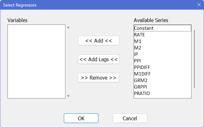
You can add variables from the “Available Series” list to the regression by: double-clicking on a series name in the “Available” list; selecting one or more series and clicking the  button; or using the  button to add lagged variables to the regression list

 

For this regression, add CONSTANT, IP, M1DIFF, and PPISUM to this list of regressors (CONSTANT is a special built-in series name, used to include a series of ones in a regression):

 

 

Click “OK” to close the list. The main dialog should now look like this:

 

 

Click “OK” to run the regression. The Wizard will generate the instruction below. (Note that in the saved example file, we have used Edit—To Lower Case to replace the upper case with lower. The Wizards generally use upper case to help show what they were used to generate).

 

LINREG RATE

# Constant IP M1DIFF PPISUM

 

LINREG is the standard instruction for estimating linear regressions. Here, it regresses the dependent variable RATE on the independent variables IP, M1DIFF, and PPISUM, and includes a constant term (intercept) in the regression.

 

The line beginning with the # symbol is called a supplementary card. Supplementary cards are used with many instructions to supply additional information to an instruction—usually lists of series or equations. Supplementary cards always begin with the # character.

 

The results will be somewhat different from those shown in the text book, because the data are not identical due to revisions made since Pindyck and Rubinfeld extracted their data. LINREG estimates using ordinary least squares (OLS).

 

This is the output produced by this:

 

Linear Regression - Estimation by Least Squares

Dependent Variable RATE

Monthly Data From 1959:04 To 1996:02

Usable Observations                       443

Degrees of Freedom                        439

Centered R^2                        0.2526958

R-Bar^2                             0.2475890

Uncentered R^2                      0.8717009

Mean of Dependent Variable       6.0806546275

Std Error of Dependent Variable  2.7714419161

Standard Error of Estimate       2.4039938631

Sum of Squared Residuals         2537.0628709

Regression F(3,439)                   49.4816

Significance Level of F             0.0000000

Log Likelihood                     -1015.1499

Durbin-Watson Statistic                0.0816

 

    Variable                        Coeff      Std Error      T-Stat      Signif

**********************************************************************************

1.  Constant                     2.11841571   0.42030566      5.04018  0.00000068

2.  IP                           0.06417324   0.00768853      8.34662  0.00000000

3.  M1DIFF                      -0.04183328   0.01485687     -2.81575  0.00508547

4.  PPISUM                      58.26459284   8.01033322      7.27368  0.00000000

 

Loading into a Report Window

For many uses, particularly when you’re examining several possible models, the text output shown above is most convenient, since the output from all the models will be together in a single file. However, when you’ve finally settled on a specification, this isn’t what you want, since the format for the numbers is fixed the way you see them in the editor. You could round them yourself and type them into a document, but we’re trying to show you how to avoid that.

 

Instead, you can reload the same information into a Report Window. To do that, you can open the Window—Report Windows submenu and select the “Linear Regression–Least Squares” report. The Report Windows list shows (up to) the last fifteen “reports” generated, with the most recent ones at the top of the list.

 

Once you’ve reloaded the regression into a window, you can use the Report Window operations for reformatting numbers and copying the information for use in word processors. For example, you can select sections of the report and use View—Change Layout to change the number of decimal places for the selected numbers, and then use Edit—Copy or File—Export to get the results into another program or file.

 

In addition to reports generated by RATS instructions like LINREG, you can also create your own reports with the precise information that you want. That’s a more advanced, but very useful, feature covered in "Reports".

 

Estimating the Second Equation

Now let’s estimate equation \eqref{eq:started_PandReq2}. If you select the Statistics—Linear Regressions operation again, you’ll see the same dialog box as before, loaded with the settings from the last regression. To modify the equation, you can either edit the regressor list directly in the “Explanatory Variables” box, or you can click on the  button to use the regressors dialog box. If you use the regressors dialog box, use  to delete M1DIFF and PPISUM from the list. Add GRM2, and use  to add lag 1 of GRPPI. The regressor list should look like this:

 

constant ip grm2 grppi{1}

 

Click “OK” in the main regressions dialog box to execute the regression.

 

Here’s the command that is generated and the output:

 

LINREG RATE

# Constant IP GRM2 GRPPI{1}

 

 

Linear Regression - Estimation by Least Squares

Dependent Variable RATE

Monthly Data From 1959:03 To 1996:02

Usable Observations                       444

Degrees of Freedom                        440

Centered R^2                        0.2215769

R-Bar^2                             0.2162694

Uncentered R^2                      0.8660034

Mean of Dependent Variable       6.0733783784

Std Error of Dependent Variable  2.7725545963

Standard Error of Estimate       2.4545026092

Sum of Squared Residuals         2650.8165458

Regression F(3,440)                   41.7484

Significance Level of F             0.0000000

Log Likelihood                     -1026.6780

Durbin-Watson Statistic                0.1730

 

    Variable                        Coeff      Std Error      T-Stat      Signif

**********************************************************************************

1.  Constant                     1.20988109   0.52637190      2.29853  0.02199968

2.  IP                           0.06525852   0.00727000      8.97641  0.00000000

3.  GRM2                       136.19299812  34.77735583      3.91614  0.00010426

4.  GRPPI{1}                   101.94478474  17.17615119      5.93525  0.00000001

 

Range Parameters

Our first model used M1DIFF, which isn’t defined for the first three periods, since it uses lag 3 of M1. This second model replaces that with GRM2, which only drops one point; the range for this regression is determined by the one-period lag of GRPPI which isn’t defined until 1959:3. When you execute the LINREG, RATS will scan the data, determine that 1959:4 is the earliest possible starting point for the first regression and 1959:3 is the earliest possible date for the second. Its ability to handle such entry range issues automatically is a very powerful feature.

 

With time series models with lags, you need to be somewhat careful about doing comparisons of estimates based upon different ranges, as we have with these two. The statistics which are sums (rather than averages) are especially affected by this: here the “Sum of Squared Residuals” and the “Log Likelihood”, which shouldn’t be compared when computed over different ranges.

 

Even the other statistics, which are based on averages, are only somewhat comparable. If we were seriously interested in choosing between these (we aren’t, since both have very low Durbin-Watson statistics, so neither is a serious model for the interest rate), we should re-estimate the second regression over the same range as the first. While you can redo the Regression Wizard, and reset the “Sample Start” box, it’s simpler to just edit the instruction and re-estimate it. We can change it to

 

linreg rate 1959:4 *

# constant ip grm2 grppi{1}

 

Almost any instruction which operates across a set of data allows you to give an explicit range, or to let RATS figure it out. Here, we need to override the standard handling, which for a regression uses the maximum range possible with the series involved. The estimation range has start and end parameters; we’re fine with the end being the automatic value, which is what the * means. What we need to override is the start, which we do by giving the start date of 1959:4. If we wanted to restrict the top end of the regression range (say to the end of 1992), we would use

 

linreg rate 1959:4 1992:4

# constant ip grm2 grppi{1}

 

If we wanted to restrict the end of the range, but use as much data as possible at the start, we would use:

 

linreg rate * 1992:4

# constant ip grm2 grppi{1}

 

If you want to use the default for both range parameters, you can just leave them out if nothing comes after them. If there are trailing parameters, you either have to use * *, or you can also use the shorthand / to cover both. For instance, LINREG has a fourth parameter (for the generated residuals), so if we wanted to estimate this over the full range and save the residuals into the series U, we could use

 

linreg rate / u

# constant ip grm2 grppi{1}

 

While not common with time series data, it’s also possible to skip entries out of the middle of the data set. We’ll look at that in Example Five, which works with cross-section data.

 

Learn More: Procedures

Learn More: Reading Data

Learn More: Annotated Regression Output

Learn More: The Series Window

Learn More: Arithmetic Expressions

Copyright © 2025 Thomas A. Doan